Time series model types
This article demonstrates how you can represent a number of well-known time series models as Dynamic Bayesian networks (DBN).
While you can represent more complex models with a DBN, it is useful to understand how simple time series models relate.
You can extend well known models by adding additional structure. For example a simple extension would be a mixture of Hidden Markov models.
- For an introduction to building time series models with Bayes Server please see our article on Dynamic Bayesian networks
- As Bayes Server supports learning both multi-variate time series, and multiple (multi-variate) time series, an import learning options is TimeSeriesMode which can be Pinned or Rolling.
- Many of the models described below make use of Multi-variate nodes.
- All models are multi-variate and handle missing data
- Time series models in Bayes Server can include both temporal (time series) and contemporal (non time series) variables
- Bayes Server supports time series Anomaly detection
- Bayes Server supports most probable sequence for discrete time series (an extension of the Viterbi algorithm)
Dynamic Bayesian network
Before we provide examples or well-known models, here is an example of a simple Dynamic Bayesian network.
Vector Auto regressive model
A multivariate auto regressive model, known as a vector auto regressive model.
This is one of the simplest DBNs you can create
With only a single variable, this is a probabilistic version of linear regression. The multi-variate version is equivalent to a probabilistic version of a Vector auto-regressive model.
Even a simple model such as this, represented as a Bayesian network has significant advantages, such as handling missing data, and model verification (if data is anomalous, should we trust a prediction Anomaly detection)
N-Order Markov model
The image below shows a first order Markov model, also known as a Markov chain.
Again, since a Bayesian network is probabilistic this model can handle missing data.
By adding addition temporal links you can represent an N-order Markov chain.

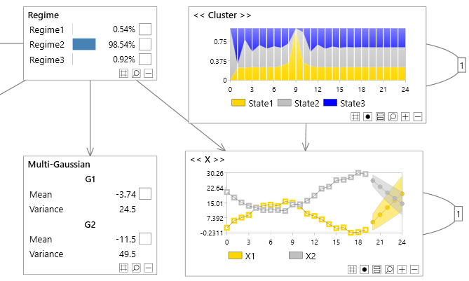
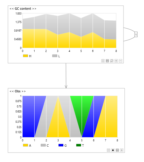
Hidden Markov model
An Hidden Markov model can be represented as a Bayesian network shown below.
- The example below uses a multi-variate node
- The transition node is called a Latent Variable
- You could also use separate nodes for the observed variables, and in a Bayesian network they can have links between them.
- In a Bayesian network you can mix discrete and continuous nodes
- You can have missing data
- A Bayesian network is not limited to this structure.
- Use max-propagation if you need the most probable sequence (Viterbi algorithm)
Hidden Markov models have the advantage that the latent (transition node) allows information to flow through many time steps.
Hidden Markov models are good at predicting transition variables, but are somewhat crude at predicting observation variables. This is because all information must flow through the latent discrete transition variable, and hence nuanced continuous adjustments are lost. (Bayesian networks do not suffer from this limitation ) .
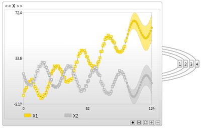
Time series clustering
Also known as a mixture of auto regressive models.
Unlike Hidden Markov models, Time series clustering models can handle nuanced continuous predictions, however they lack the ability to handle information from unlimited history. This is because all time-series information flows through the observation node.
Bayesian networks support models with latent nodes (discrete or continuous) such as an Hidden Markov model, Time Series clustering models, or a hybrid. Bayesian network structure can handle both or more exotic models.
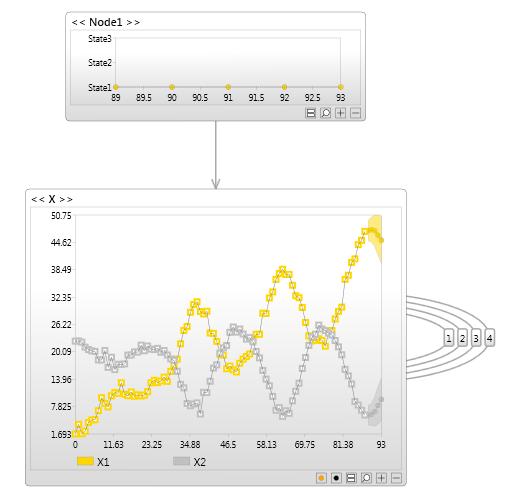
Kalman Filter
A Kalman filter model is similar to an Hidden Markov model. The only difference is that the latent node is continuous instead of discrete.
Once again, with Bayesian networks you are not limited to this structure.
Exact & approximate inference
If a time series model has more than one temporal path, then moving beyond short term predictions may require approximate inference ( which Bayes Server supports). In fact you can use exact inference for short term and approximate inference for long term.
By temporal path, we mean how information can flow into the future. For example an Hidden Markov model has only one temporal path (via the hidden/latent variable). The same is true for Kalman filters.
With a Mixtures of Time Series models information can only flow info the future via the observed node.
A model that has temporal links with both latent variables and observed variables (e.g. a hybrid between an Hidden Markov model and a Mixture of time series models) has multiple paths.
When multiple paths exist, exact inference (while generally preferred with Bayesian networks) is fine for a number of steps, becomes hard beyond a a certain number of time steps.