Mixture models

This article describes how mixture models can be represented using a Bayesian network.

What are mixture models?

Mixture models are a type of probabilistic model which are capable of detecting similar groups of data. Each similar group is known as a cluster. The process of grouping similar data is known as clustering, segmentation or density estimation.

• Clustering - a term often used, because each group of similar data is called a cluster.
• Segmentation - a term often used when the groups are used to separate entities such as customers for the purposes of marketing.
• Density estimation - a term often used, because a probabilistic model such as a mixture model, estimates a probability density function (pdf).

In machine learning terminology, a mixture model is termed an unsupervised learning technique. This is because unlike classification, in which training is focused around predicting outputs based on inputs, a mixture model detects natural groupings of input data without regard to output variables. Interestingly, although not the most common usage, we will see later that a mixture model can be used for prediction.

Image 1 shows two dimensions of a mixture model. Each ellipse represents a cluster in the mixture model, and the data that was used to train this model is plotted to show how well the model represents the data.

The term mixture model is used because the model is a mixture (collection) of probability distributions. The model depicted in Image 1, is a mixture of Gaussians.

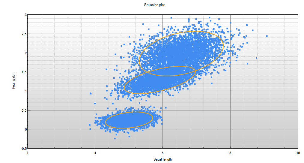
Image 1 - plot of a Gaussian mixture model with training data

Usage

Mixture models have a wide range of uses. Since a mixture model is a probability density function, we can perform the same tasks as we can with other probability distributions, such as a Gaussian. In fact most mixture models are a mixture of multivariate Gaussians.

Data exploration

Mixture models are useful for identifying key characteristics of your data, such as the most common relationships between variables, and also unusual relationships.

Segmentation

Because clustering detects similar groups, we can identify a group that has certain qualities and then determine segments of our data that have a high probability of belonging to that group.

Anomaly detection

Unseen data can be compared against a model, to determine how unusual (anomalous) that data is. Often the log likelihood statistic is used as a measure, as it tells you how likely it is that the model could have generated that data point. While humans are very good at interpreting 2D and 3D data, we are not so good in higher dimensional space. For example a mixture model could have tens or even hundreds of dimensions.

Prediction

Although Mixture models are an unsupervised learning technique, we can use them for prediction if during learning, we include variables we wish to predict (output variables).

This can be done in two ways. The first allows output variables to take an active part in learning, the second simply gathers statistics for the output variables, but does not let them change the model. Either way, once we have a model that includes our output variables, we can make predictions in the standard way.

It is important to note however that since Mixture models are an unsupervised techniques, the learning process is not concerned with creating a model that is good at predicting your outputs from inputs. It is only concerned with finding natural groupings in the data. That said, Mixture models can be surprisingly good at predictions, and the predictions are made without assumptions made by the modeler as to how the inputs relate to the outputs.

Mixture models as Bayesian networks

Mixture models are simple Bayesian networks, and therefore we can represent them graphically as shown in Image 2.

Image 2 - Bayesian network mixture model

The node named cluster is a discrete variable, with a number of discrete states, each representing an individual cluster. Each state has a probability associated with it, which tells us how much support there was for a cluster during learning. The node named X contains four continuous variables X1, X2, X2 and X4. The distribution assigned to node X is a multivariate Gaussian distribution, one for each state of node cluster. Therefore our Mixture model is a mixture (collection) of multivariate Gaussians. Since this is just a Bayesian network, the probability distribution of the model is the product of the probabilities of each node given their parents, i.e. P(Cluster)P(X1,X2,X3,X4|Cluster).

There are other ways a Mixture model can be represented as a Bayesian network. Image 3 shows a model which is equivalent to the model in Image 2, however only has a single variable per node.

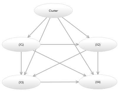
Image 3 - Alternative Bayesian network mixture model

Image 4 shows a Mixture model in which the probability of each continuous variable is independent of the other continuous variables given the cluster. This model has fewer parameters, however cannot represent the rotations of ellipses shown in Image

1. A model such as this is termed a diagonal model, because if you constructed a multivariate Gaussian over the continuous variables, all values of the covariance matrix would be zero, except for the diagonal variance entries.

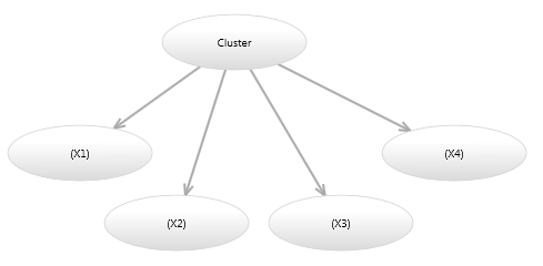
Image 4 - Diagonal Bayesian network mixture model

Unlike some clustering techniques where a data point only belongs to a single cluster (hard clustering), probabilistic mixture models use what is known as soft clustering, i.e. each point belongs to each cluster with a probability. These probabilities sum to 1.

The node named cluster, is sometimes called a latent node. This is because we do not have data associated with it during learning.

Learning

Usually the parameters of a model are learned from data. For the model shown in Image 1, the task is to estimate the probability (weight/support) of each cluster and also the mean and covariance matrix of X for each cluster. Because there is no data associated with the latent cluster node, we are actually learning with missing data. The Expectation Maximization (EM) algorithm is often used to determine the required parameters using an iterative approach.

Usually a model is learned multiple times, with different initial configurations for the parameters, since a mixture model has multiple local maxima (unless there is only one cluster).

Extending mixture models

Mixture models can be extended within the Bayesian network framework to create models with additional structure. It is interesting to point out, that even with additional structure, the joint distribution of the model will still be a Mixture Model, however the additional structure allows us to use a compact probability distribution leading to increased performance, reduced memory consumption and greater interpretability when viewing the model graphically.

Temporal mixture models

If we add temporal links to a mixture model, we can create a number of useful models. An example of this is the Hidden Markov Model (HMM) shown in Image 5, which can be used for modeling time series data.

Image 5 - Bayesian network hidden Markov model

The link labeled 1 in Image 5, indicates that the link has order 1, which means that the Cluster Node is linked to itself in the next time step. This is easier to see if we unroll the model for a few time steps, as shown in Image 6.

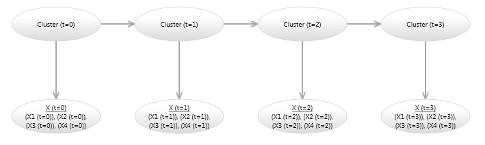
Image 6 - Bayesian network hidden Markov model (unrolled)

In the same way that we can extend a mixture model with additional structure, we can extend temporal models with additional structure.

Summary

Mixture models are a very popular statistical technique. We have shown how a simple Bayesian network can represent a mixture model, and discussed the type of tasks they can perform. We have also suggested ways in which mixture models can be extended within the Bayesian network paradigm, including time series models.