Latent variables - what are they and why are they useful
In this article we explain what latent variables are, and why they are so important.
A column of missing data
Consider the data in the following table. The third column 'Device Type' has no values. If we built a model with 3 variables 'Asset', 'Sensor', and 'Device Type' , then 'Device Type' is a latent variable because there is no data in that column. Another way of putting it, is that the variable is unobserved or missing. I.e. we are unable to observe the data directly for some reason. Perhaps it is too expensive to collect the data, it was not recorded, or we do not have direct access to the process generating the data we can observe.
| Asset | Sensor | Device Type |
|---|---|---|
| A | 176 | |
| C | 163 | |
| A | 185 | |
| B | 160 | |
| C | 158 | |
| A | 180 | |
| ... | ... | ... |
Given the data above, even though the 'Device Type' column has no data, we can still build a model. We will need to provide it with the number of possible values (states) the 'Device Type' column can take, or use an algorithm to determine the best number (see Clustering and Cluster Count) In this case we could build a model with two possible states, and the model will automatically determine the relationship between the 3 variables using an iterative algorithm called the EM algorithm.
To build a model, we do not actually need to have a column of empty data in our database table, but it is useful to imagine that we have.
This is an example of a discrete latent variable, because we have specified that the 'Device Type' column can take one of a number of states.
In general we may not know in advance how many states the discrete latent variable should have, so we might build a number of models each with a differing number of states and compare them using metrics on test data such as accuracy, lift score or log-likelihood.
Cross validation is a useful technique to measure the performance of models on unseen data.
Visualizing discrete latent variables
Now consider the data below. Again we have 3 columns of data which we can model with 3 variables, one for each column 'X', 'Y' and 'Cluster'. We will again assume that the 3rd column is a discrete latent variable, and we will call it 'Cluster' because this time we are not sure what the variable means but we do know that we want to group (cluster) similar rows of data together. We could have called the 'Device Type' column in the previous example 'Cluster', as again that is grouping similar rows together. Sometimes however we can give the latent variable a name and may even be able to label the states with a meaningful name after learning.
| X | Y | Cluster |
|---|---|---|
| 0.176502224 | 7.640580199 | |
| 1.308020831 | 8.321963251 | |
| 7.841271129 | 3.34044587 | |
| 2.623799516 | 6.667664279 | |
| 8.617288623 | 3.319091539 | |
| ... | ... | ... |
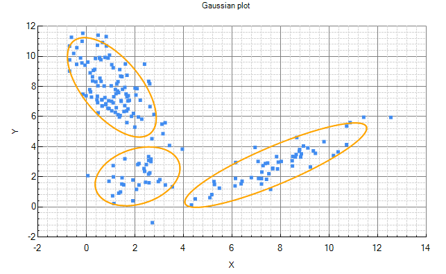
If we learn a model (perhaps using cross validation) we may find that the best model has 3 states for the 'Cluster' variable, i.e. the model found 3 clusters/groups of data. What has happened is that the learning algorithms has automatically grouped our data into 3 different groups of similar data called clusters. If we plot the data and the model, each ellipse in the chart below corresponds to one of the 3 states in our discrete latent variable 'Cluster'.
This particular model in Bayes Server would look like this.
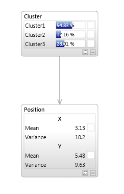
The 'Cluster' variable has 3 states, meaning that we have 3 different groups (clusters). We then have a multivariate Gaussian over X and Y for each of those states corresponding to an ellipse in the chart.
This kind of model is sometimes called a generative model, because we could generate data from the model by first randomly selecting a cluster state. The chosen cluster state corresponds to one of the ellipses in the chart above. From that ellipse which is a multivariate Gaussian we can sample X and Y. If we repeat this process many times, we have a data set sampled from the model.
Why is this important?
Consider the X-Y data in the plot above. We only have 2 columns of data, X and Y, so we might have decided to start by building a model with just two variable called 'X' and 'Y'. Perhaps we use a Gaussian for these variables. The problem with this is that we then only have a single ellipse to fit to our data. This will produce a poor model because clearly there are different groupings in the data (clusters) even though we do not have this information in the data. We can fix this by adding a discrete latent variable. This is the same as adding a column of missing data which can take different discrete values. I.e. we can now fit multiple ellipses to our data as shown in the chart above.
Discrete latent variables are powerful because we can model complex patterns that we do not have complete data for. If we are modeling data from a complex system , instead of attempting to build a physics model of the entire process, we can use a data driven approach and build a model from the data. Because the data we can observe (record) does not always provide all the information we need to model the system adequately we can use latent variables to give us more expressive power.
Multiple latent variables
We are not restricted to a single latent variable in a model. We can have as many as we like, each one corresponding to a column of empty data.
As with normal variables in a Bayesian network, we can connect these latent variables to each other and standard variables.
Deep belief networks
A Deep Belief network is an example of a model which has multiple latent variables, typically boolean.
An example is a model which has a number of leaf nodes (variables) which correspond
to observed facts. For example each leaf node might represent a word, with states {True, False} to indicate whether that word appeared in a portion of text or document.
The model also includes a number of additional layers of boolean latent variables, creating a hierarchy of concepts.
For example, if the leaf nodes represent words, the next layer up may contain boolean latent variables which tell us when those words appear together.
The next layer up again, may tell us when those phrases appear together, and so on, forming a hierarchy.
Continuous latent variables
Continuous latent variables are the same as discrete latent variables except that the variable we use for our missing column of data is continuous instead of discrete.
In fact when using continuous latent variables it is common to have multiple columns of missing data, i.e. multiple continuous latent variables.
As with discrete latent variables the continuous columns just represents data that was not observed. We can however use a learning algorithm to determine the relationships between the observed variables and unobserved (latent) variables.
An example of a model that uses continuous latent variable is when we want to reduce the dimensionality of a data set. Perhaps our observed data has 100 continuous columns of data but we think that much of that data is highly correlated because it is the result of a simpler underlying process, and we wish to pick out just the important patterns. To do this we can use a model with continuous latent variables to represent the underlying process we wish to capture. A simple example of this is shown in the model below.
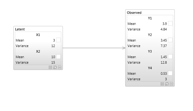
A model can contain both discrete and continuous variables.
Latent variables in time series and sequence models
Just like the models seen earlier, time series models and sequence models can and often do contain discrete or continuous latent variables.
In the earlier example where we needed more than one ellipse (Gaussian) to model our data adequately, the same is true for time series or sequences. Instead of having a single ellipse to model the relationship between a time series variable X and itself at a previous time (auto correlation), or X and another time series variable Y (cross correlation) we can use multiple ellipses to give us more expressive power.
What we are saying is that our time series (with one or more series) does not always behave the same, just like we had different groups in our cluster model charted earlier.
Some of the models we can represent with latent variables in temporal Bayesian networks (Dynamic Bayesian networks) are Hidden Markov Models, Kalman Filters, Sequence clustering, mixtures of auto regressive models, mixtures of vector auto regressive models. There are many more model types that can be constructed using Bayesian networks, however they do not all have well recognized names.