Dynamic Bayesian networks - an introduction
What are dynamic Bayesian networks?
Dynamic Bayesian networks extend standard Bayesian networks with the concept of time. This allows us to model time series or sequences. In fact they can model complex multivariate time series, which means we can model the relationships between multiple time series in the same model, and also different regimes of behavior, since time series often behave differently in different contexts.
If you are not familiar with standard Bayesian networks we recommend you first read our Bayesian network article.
We will use the terms Dynamic Bayesian network (DBN), temporal Bayesian network, time series network interchangeably.
Note that the term Dynamic means we are dealing with time, not that the model necessarily changes dynamically.
Some important features of Dynamic Bayesian networks in Bayes Server are listed below.
- Support multivariate time series (i.e. not restricted to a single time series/sequence)
- Support for time series and sequences, or both in the same model.
- Anomaly detection support
- Complex temporal queries such as P(A, B[t=8], B[t=9], C[t=8] | D, E[t=4])
- Most probable sequence
- Prediction, filtering, smoothing
- Latent temporal variables (discrete and continuous)
- Mix temporal and non temporal variables in the same model
- Parameter learning of temporal models
- Structural learning of temporal models
- Log likelihood - useful for time series anomaly detection
Figure 1 shows a simple dynamic Bayesian network predicting a multivariate time series into the future.
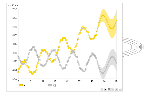
Figure 1 - a simple bivariate dynamic Bayesian network
Auto, cross & partial correlation
In general time series modelling the terms Auto, cross & partial correlation are often used.
- Auto correlation - correlation between a variable at different times (lags)
- Cross correlation - correlation between different time series
- Partial correlation - correlation between the same or a different time series with the effect of lower order correlations removed.
Dynamic Bayesian networks can capture all the above types of correlation and model even more complex relationships, as these correlations can be conditional on other variables (temporal or non-temporal) and on latent variables (described later) and models can include both discrete and continuous variables.
Do I need a temporal model?
Just because data is recorded sequentially in time does not always mean you have to use a time series model (DBN).
For some tasks, a standard Bayesian network may perform very well, and the added complexity of a temporal model may not be justified.
In these cases, it is good practice to create a non-temporal model first for comparison, before developing a Dynamic Bayesian network.
As explained in more detail later you have to be careful when creating test and validation datasets from time series data, as the data is usually not IID (Independent and identically distributed).
Variable contexts
Bayes Server has natively supported the concept of time, and temporal models from the first release.
Each distribution in Bayes server contains a number of variables.
A distribution can actually have zero variables, but is not then strictly a distribution.
In a standard Bayesian network with variables {A,B,C,D,E} some example distributions are shown below:
- P(A)
- P(A,B)
- P(A|B)
- P(A,B|D,E)
A distribution in Bayes Server actually has a collection of VariableContexts rather than Variables. Each VariableContext holds
a reference to a variable, but can also have other information such as time.
Variable contexts allow us to construct time aware distributions, some examples of which are shown below.
We use t as shorthand for time, so t=5 means at time 5. All times are zero based, so t=0 is the first time step.
- P(A[t=5])
- P(A[t=5], A[t=6]])
- P(A[t=2], B)
- P(A[t=2], B, C[t=2], C[t=3])
- P(A[t=2] | P(A[t=1])
Note that distributions can have a mixture of temporal and non-temporal variables. A temporal variable can appear in the same distribution more than once only if the associated times are different.
Temporal nodes
Dynamic Bayesian networks can contain both nodes which are time based (temporal), and those found in a standard Bayesian network. They also support both continuous and discrete variables.
Multiple variables representing different but (perhaps) related time series can exist in the same model. Their dependencies can be modeled leading to models that can make multivariate time series predictions. This means that instead of using only a single time series to make a prediction, we can use many time series and their interrelations to make better predictions.
Note that a Bayesian network in Bayes Server becomes a Dynamic Bayesian network as soon as you add a temporal node.
Initial & terminal nodes
There are a few special kinds of nodes.
Initial nodes only ever connect to temporal nodes at t=0.
Terminal nodes only ever connect from temporal nodes at the final time (which can vary from case to case).
Temporal links
In Bayes Server a temporal link is much like a standard link in a Bayesian network except for the following:
- It has an associated order (lag)
- It can only link two temporal variables
- It can link a node to itself
The order of a temporal link is sometimes referred to as a lag.
As an example, a temporal link with order 2 from a node A to another node B, means that A links to B in the future (two time intervals/steps) later.
Or put another way, B has a link from A in the past (two time intervals/steps in the past).
Note that a link can be added between two different temporal nodes at the same time (t=0), and you can link non-temporal nodes to temporal nodes, but not the other way round.
Temporal Distributions
Temporal nodes in a Dynamic Bayesian network typically require more than one distribution to be fully specified.
These distributions can be learned from data as explained later, or specified manually.
The reason for this is that as a time series evolves, different distributions come into play. For example at t=0 there is no previous data, whereas at t=5 there are 5 previous points.
If a model had a temporal link of order 5, it would have previous data at t=5, but if it also had a temporal link of order 10, it would not yet have previous data from that link. Therefore separate distributions are used to accommodate different incoming data.
Often only a couple are required to cover all scenarios, and once t >= max order, the same distribution is used thereafter.
Multi-variable nodes
As with standard Bayesian networks, Dynamic Bayesian networks in Bayes Server support multiple variables in a node (multi-variable nodes).
This is especially useful for temporal models as their structure is vastly simplified, inference is often faster and it can be easier to interpret the parameters.
Unrolling
A useful way to understand a dynamic Bayesian network, is to unroll it. Unrolling means converting a dynamic Bayesian network into its equivalent Bayesian network.
Note that in Bayes Server unrolling serves no other purpose other than being useful to understand the structure of a dynamic Bayesian network. Unrolling is not necessary to perform predictions (queries) and we do not unroll the network internally during inference.
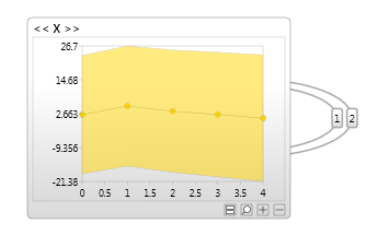
Figure 2 - a simple dynamic Bayesian network
Figure 2 shows a simple dynamic Bayesian network with a single variable X. It has two links, both linking X to itself at a future point in time. The first has the label (order) 1, which means the link connects the variable X at time t to itself at time t+1. The second is of order 2, linking X(t) to X(t+2). Figure 3 shows the same network unrolled for 5 time slices, which makes understanding the structure easier.
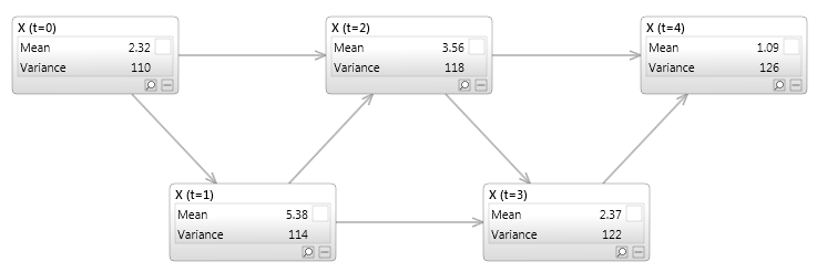
Figure 3 - a simple dynamic Bayesian network unrolled for 5 time slices
Note that the two networks are not actually equivalent unless some of the unrolled nodes were able to share distributions.
Discrete time vs continuous time
Dynamic Bayesian networks are based on discrete time. Discrete time and continuous time are different ways of modeling variables that change over time.
Discrete time considers data at separate points in time, which is often how time series data is stored (e.g. data from a sensor is recorded once a minute). Continuous time on the other hand consider values to be continually changing, and is often used in theoretical models such as those found in Physics or options pricing.
Temporal Evidence
Evidence is what we know about the current value of variables, when we wish to make predictions. Evidence on a standard node in a Bayesian network, might be that someone's Country is US, or someone's age is 37, however for a time based (temporal) node in a dynamic Bayesian network, evidence consists of a time series or a sequence. For example X might have evidence {1.2, 3.4, 4.5, 3.2, 3.4}, or Y might have evidence {Low, Low, Medium, Medium, High } which looks as follows in tabular form:
| Time | X | Y |
|---|---|---|
| 0 | 1.2 | Low |
| 1 | 3.4 | Low |
| 2 | 4.5 | Medium |
| 3 | 3.2 | Medium |
| 4 | 3.4 | High |
Zero based indexing
Times in Bayes Server are zero based, meaning that the first time step is at zero.
We often use a lowercase t as a shorthand for time, so t=5 means the sixth time step.
Missing data
As with standard Bayesian networks, Dynamic Bayesian networks natively support missing data.
You do not need to fill in or exclude records with missing data.
It can sometimes be useful to exclude columns of data which have a large percentage of missing data.
For example variables X and Y might have the following evidence in the table below.
| Time | X | Y |
|---|---|---|
| 0 | 1.2 | Low |
| 1 | Low | |
| 2 | 4.5 | |
| 3 | 3.2 | Medium |
| 4 | 3.4 | High |
Note also that Bayes Server supports both discrete and continuous temporal latent variables which are very powerful.
Non-temporal and temporal data
Since Dynamic Bayesian networks can contain both temporal and non-temporal variables, evidence can be a mixture of time series/sequence data and non temporal data.
Multivariate time series/sequences
Time series and sequence data can be multivariate, which simply means that multiple time series and sequences can be included in the same model, and their relationships modeled.
An example is given below:
| Time | Stock price A | Stock price B | Stock price C | Volatility |
|---|---|---|---|---|
| 0 | 312.4 | 104.3 | 1233.3 | Low |
| 1 | 315.6 | 107.2 | 1229.5 | Low |
| 2 | 313.8 | 110.2 | 1241.6 | Medium |
| 3 | 314.2 | 111.4 | 1241.0 | High |
| 4 | 315.2 | 109.4 | 1245.9 | High |
Hierarchical data
As well as being multi-variate, time series/sequences can be continuous like stock data or hierarchical in nature.
As an example, consider geo-spatial data generated by aircraft during flights.
| Flight | Carrier | Time | Lat | Lon | Altitude |
|---|---|---|---|---|---|
| 0 | American Airlines | ||||
| 0 | 40.7 | -73.9 | 0.0 | ||
| 1 | 45.1 | -62.1 | 40121.5 | ||
| 2 | 47.2 | -48.1 | 40255.6 | ||
| ... | ... | ... | ... | ||
| 12 | 51.5 | 0.45 | 0.0 | ||
| 1 | Southwest | ||||
| 0 | 28.5 | 81.4 | 0.0 | ||
| 1 | 34.6 | -91.2 | 37142.1 | ||
| ... | ... | ... | ... | ||
| 6 | 33.9 | 118.4 | 0.0 |
Note that different flights have different length time series / sequences.
Bayes Server can learn from both multivariate, continuous and hierarchical data.
Simple well known models
Dynamic Bayesian network models are very flexible and hence many of the models built do not have well known names.
However some very simple Dynamic Bayesian networks have well known names, and it is helpful to understand them as they can be extended.
Some examples are:
- Hidden Markov model (HMM)
- Kalman filter (KFM)
- Time series clustering
- Auto regressive model
- Vector auto-regressive model
With Dynamic Bayesian network you can extend these. For example:
- Hybrid HMM and time series clustering
- Mixture of Kalman filters
- ...
Parameter learning
Parameter learning works in a similar way to standard Bayesian networks.
Time series mode
One key option is the TimeSeriesMode which can be set to Rolling or Pinned.
In rolling mode it is assumed that the beginning of the series (single or hierarchical) has no particular significance.
For example a particular stock time series falls into this category, as the beginning is just when the series was first recorded.
In rolling mode lower order distributions learn from all the data.
In Pinned mode, the beginning of the series is the start point. An example being the beginning of the flight.
In Pinned mode lower order distributions only learn from the data until a higher order distribution takes over.
If in doubt, we advise using Rolling mode.
Structural learning
Structural learning works in the same way to standard Bayesian networks, except that both temporal links and non-temporal links are discovered.
While structural learning is a great tool, often the structure can be defined using a well known model type and extended.
Predictions
Dynamic Bayesian networks extend the number of prediction types available.
Prediction, filtering, smoothing
- Predicting the value of variables at future time steps is known as Prediction
- Predicting the value of variables that are unobserved (do not have evidence) at the current time is known as Filtering.
- Predicting the value of unobserved variables in the past is known as Smoothing.
A query could even span past, current and future times, which demonstrates the flexibility of the system.
As with predictions in a standard Bayesian network, we get not only the predicted values, but also variances for continuous variables and probabilities for discrete states, indicating the uncertainty in the prediction.
As mentioned earlier, joint queries can include both temporal and non-temporal variables, can include multiple temporal variables, and the same temporal variable at different times.
Unrolling not required
Unlike many systems, Bayes Server natively supports the concept of time and also does not need to unroll a dynamic representation to a standard Bayesian network before performing inference.
One reason this is important is that time series evidence can vary in length
Most probable sequence
As with standard Bayesian networks, Dynamic Bayesian networks can use the Most probable explanation feature to find the Most probable Sequence.
This is similar to the use of the Viterbi algorithm with Hidden Markov models, however is more general.
Exact & approximate inference
Both exact and approximate algorithms can be used with time series and sequence DBNs. An example of when approximate inference is useful is when a temporal model has multiple temporal paths and longer range predictions are required.
Hybrid inference
Hybrid inference is a term we use when exact inference is used for short term predictions and then approximate inference is used for longer range predictions.
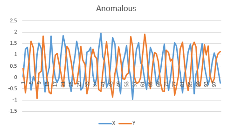
Anomaly detection
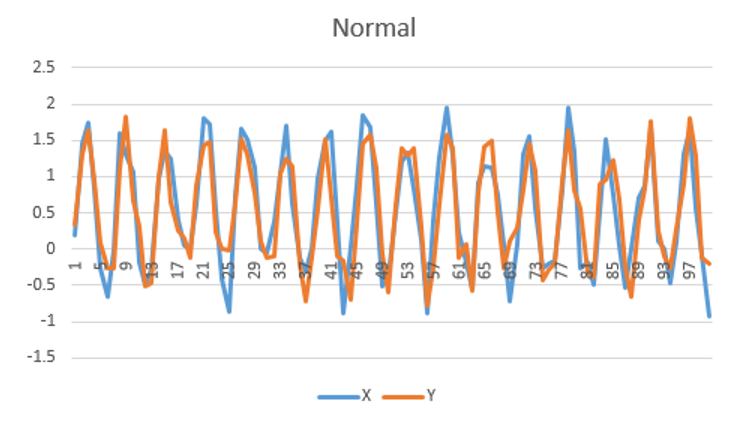
As with standard Bayesian networks, we can make use of the Log-likelihood to determine if new data series are anomalous. This is an example of time series anomaly detection.
A very simple example is shown below, but the data and models can be much more complex.
Temporal Latent variables
As with standard Bayesian networks, Dynamic Bayesian networks can contain one or more temporal latent variables to model hidden patterns.
As an example consider a DBN which models the relationship between multiple time series. The relationships between the time series may vary under different conditions. If we know (have data for) these conditions, we can include them explicitly in the model, however if not, a discrete temporal latent variable will automatically uncover these patterns. This is similar to a mixture model (cluster model), except now we have a mixture of time series models (time series clustering).
Latent variable can model complex patterns, and are similar to hidden layers in a Neural network / deep learning.
Bayes Server supports the following:
- Discrete temporal latent variables (as found in a Hidden Markov model, but DBNs can be more complex)
- Continuous temporal latent variables (as found in a Kalman Filter model, but DBNs can be more complex)
- Mixed temporal and non-temporal latent variables
- Multiple temporal latent variables
Numerical stability
Many years of research have gone into the numerical stability of Bayes Server's algorithms, and in particular for time series modeling.
Underflow (and sometimes overflow) is a particular issue with Dynamic Bayesian networks, as you are often multiplying a series of very small number together. We use a number of sophisticated techniques to avoid these issues.
Test sets for non IID data
Care should be taken when creating test and validation datasets from time series data, as the data is usually not IID (Independent and identically distributed).
As an example, consider 3 points of consecutive data, and the training set includes the first and last, while the test set includes the middle point. As the points are highly correlated in time, it is very easy for an algorithm to over-fit, and report a very high accuracy on the test set when the model is actually a very poor fit.
To avoid this, training and test sets can be constructed from blocks of consecutive data.