Multi variable nodes
Introduction
Typically, a node in a Bayesian network represents a single variable. However, Bayes Server also allows a node to contain more than one variable while retaining the same functionality. We call such a node a Multi Variable Node (MVN). The approach differs from simply using vector-valued variables, and has the following advantages.
- Graphical simplicity
- Alternative parameterization/semantics
- Often leads to increased performance
Importantly, an MVN node can have missing data on some of its variables, and queries can be performed at the granularity of a variable.
For example, if a node was made up of the variables {A,B,C}, we could set evidence on A, leaving B
and C missing, and then calculate P(B,C).
In addition, queries can contain variables spanning multiple nodes, and if required evidence can be soft/virtual on one
or more variables within an MVN node.
Mixture model
A simple example of a Bayesian network with a multi variable node is a mixture model, shown in Figure 1, allowing parameters to be specified in terms of means and covariances, and without representing each variable as an individual node with lots of additional links complicating the graphical structure, as shown in the network in Figure 2 without the multi variable node.
We do however want to retain the ability to allow evidence to be set on some, but not all of the variables, and in the case of discrete variables, set soft/virtual evidence on them.
Note that the result of the queries between the two Bayesian networks are identical.
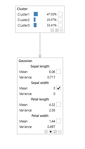
Figure 1 - mixture model with a multi variable node
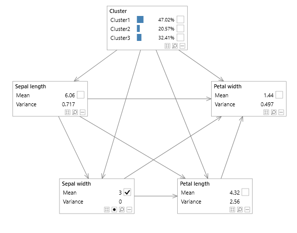
Figure 2 - mixture model without a multi variable node
Representation
We refer to a node with only a single variable as a Single Variable Node (SVN). A network with no MVN nodes is called an SVN network, whilst a network with at least one MVN node will be called an MVN network.
Multiple discrete variables
Figure 3 shows a simple Bayesian network with the nodes A and B. In this example,
node A has a single variable A1 and node B contains two variables B1 and B2 (Note that Node A could also have
contained more than one variable). As with an SVN network P(U) = P(A,B)=P(A)P(B|A) where U represents the
universe of nodes or variables. This can be written in terms of variables as follows: P(U) = P(A1, B1, B2)=P(A1)P(B1,B2|A1).
An example distribution for node B is shown in Table 1 assuming all discrete variables have the states True and False.
Note that, as with SVN networks, values sum to 1 for each parent combination, however each parent combination now
varies over both B1 and B2.
In this example sum(P(B1,B2|A1=True)) = P(B1=True, B2=True, A1=True) + P(B1=False, B2=True, A1=True) + P(B1=True, B2=False,A1=True) + P(B1=False, B2=False, A1=True) = 0.2 + 0.3 + 0.4 + 0.1 = 1.

Figure 3 - discrete multi variable node
| A1 | B2 | B1=True | B1=False |
|---|---|---|---|
| True | True | 0.2 | 0.3 |
| True | False | 0.4 | 0.1 |
| False | True | 0.15 | 0.25 |
| False | False | 0.1 | 0.5 |
Table 1 - P(B1,B2|A1)
Multiple continuous variables
Figure 4 shows an example of a network containing a node with multiple continuous variables.
Note that in Bayes Server continuous variables are identified using brackets ( ).
The probability specification of the network in terms of probabilities and densities is shown in equation 1.
 Equation 1
Table 2 shows an example distribution for node C, assuming that node A has the states True and False.
Note that all continuous distributions are Conditional Linear Gaussian distributions, and are specified in terms of Mean, Covariance and Weight (Regression coefficient).
Figure 4 - continuous multi variable node
| A1 = True | C1 | C2 |
|---|---|---|
| Mean | 3.5 | 6.1 |
| Covariance (C1) | 2.4 | 0.54 |
| Covariance (C2) | 0.54 | 1.6 |
| Weight (B1) | 0.25 | 0.34 |
| A1 = False | C1 | C2 |
|---|---|---|
| Mean | -1.5 | 0.2 |
| Covariance (C1) | 3.06 | 0.88 |
| Covariance (C2) | 0.88 | 2.45 |
| Weight (B1) | -0.54 | 0.23 |
Table 2 - P(C1,C2|A1, B1)
Factorization
The use of MVN nodes does not dictate that we must, for example, group all continuous nodes together in one node.
That would defeat the purpose of Bayesian networks in providing a compact representation of a joint probability distribution.
As shown in figure 5 we can still factorize a network as we see fit.
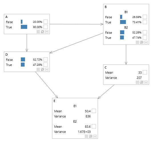
Figure 5 - Multiple MVN and SVN nodes
Constraints
MVN networks that contain continuous variables extend the rules that apply for SVN networks with continuous variables, namely:
Nodes which contain one or more continuous variables cannot have child nodes containing any discrete variables.
Vector-valued variables
Whilst there is some crossover between this approach and using vector-valued variables (i.e. variables that accept more than one value), the key differences are listed below.
- With MVN networks the fundamental unit in a query is a variable, not a node.
- MVN networks allow an MVN node to have missing values.
- MVN networks allow an MVN node to have evidence set on some variables, whilst others remain missing.
- MVN networks allow soft/virtual evidence to be set on one or more variables within an MVN node.
- A probabilistic query can contain some, but need not include all, variables from an MVN node.
- A probabilistic query can span variables in multiple MVN nodes
The following examples show a few potential queries from an MVN network. Note that temporal nodes are shown using the symbols << and >>, and t=0 (for example) denotes a temporal variable at time 0.
- P(A1,B1|A2=True,B2=True) (from figure 6)
- P(Obs1(t=0), Obs2(t=1)| Obs2(t=0)=True) (from figure 7)

Figure 6 - Vector values variable comparison
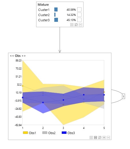
Figure 7 - Vector values variable comparison (temporal)
This is in contrast to systems supporting vector-valued variables, which will likely force either all or none of the values for each vector-valued variable to have evidence set.
Advantages
In this section we outline the advantages of the MVN framework.
Performance
Increased performance can be achieved during inference (and therefore parameter learning), using MVN networks.
The MVN Bayesian network can often be 10 times faster than the SVN equivalent in Bayes Server.
The performance improvements tend to be down to the following:
- Reduced elimination costs
- Fewer distributions to combine
Elimination is the process of marginalizing out variables that are relevant to a query and do not have evidence.
Algorithms that determine the order in which variables should be eliminated are sensitive to the number of nodes and links
in a network.
An MVN network has significantly fewer nodes and links than its SVN equivalent, and hence elimination can be far more efficient.
During the elimination process, distributions are combined, before each elimination takes place. In an MVN network, many of the distributions have already been combined in the native network format.
The performance benefits of Bayesian networks (or dynamic Bayesian networks) that are tree structures are well known. MVN networks extend the class of networks that can be represented in their initial/native format as trees.
Using MVN networks, we often find that our native representation is already a tree, where the SVN equivalent would not be.
Clearly we could just always use the joint distribution over all variables, which would defeat the object of Bayesian networks. In practice there is a middle ground, whereby a mixture of SVN and MVN nodes is preferred.
Graphical simplicity
To illustrate the fact that MVN networks provide a much simpler and appealing graphical representation, consider the MVN network in figure 10 and the equivalent SVN counterpart in figures 11.
The SVN networks lose the visually appealing structure that Bayesian networks are popular for, whereas the MVN networks retain the simple structure which is easy to interpret.
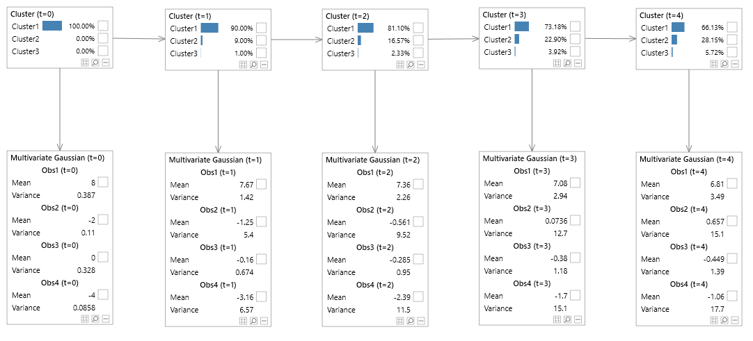
Figure 10 - Hidden Markov model (unrolled)
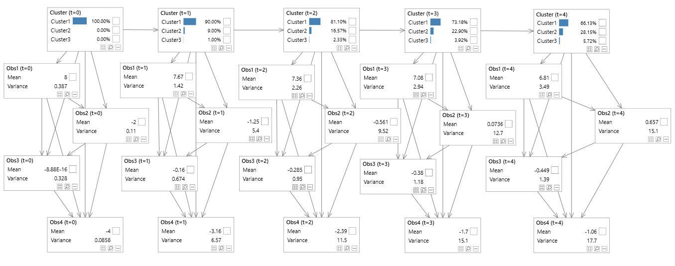
Figure 11 - Hidden Markov model (unrolled & decomposed)
Alternative parameterization
Consider the Bayesian Network shown in figure 1 which is an example of a Gaussian Mixture Model.
It was created from the ubiquitous Iris data set used in machine learning and data mining. The Cluster node contains a single
discrete variable with each state representing an individual cluster or mixture and its associated probability.
The Observations node contains 4 continuous variables; Sepal Length, Sepal Width, Petal Length and Petal Width.
The distribution associated with the Gaussian node is a mixture of multi variate Gaussians, where each Gaussian is the
position and covariance matrix of the specific cluster.
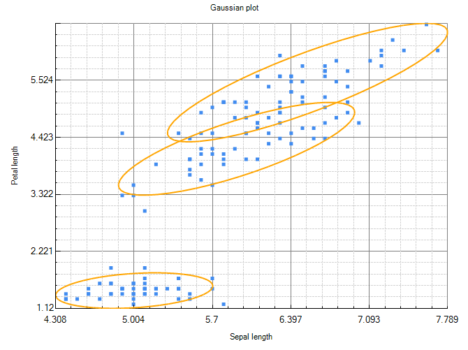
Figure 12 - MVN iris Bayesian network
Figure 12 shows two dimensions of the Mixture model. Note that the ellipses are rotated, indicating that the model includes non zero covariance entries. An equivalent SVN Bayesian network is shown in figure 2.
Had the model contained zero covariances, the ellipses would not be rotated, and we could have used the Bayesian network shown in figure 13 instead.
Not only is the MVN variant easier to visualize graphically, but provides us with an alternative, but equivalent parameterization.
This can be useful when manually defining parameter values or interpreting learned values.
Tables 3, 4, 5, 6 detail the MVN distributions, while figures 3, 7, 8, 9, 10 detail SVN equivalents (Cov = Covariance, Sl = Sepal Length, Sw = Sepal Width, Pl = Petal Length, and Pw = Petal Width).
As you would expect, the two equivalent parameterizations have the same parameter count, and the distribution for node Cluster is the same for the MVN network
and the SVN network.
Notice that the MVN distributions are parameterized in terms of covariances, whereas the SVN network is parameterized in terms of weights (regression) coefficients. Depending on the context, a Bayesian network modeler might prefer to enter weights, or enter covariances. Covariance parameterization is often preferable when the semantics of a directed link is not clear, but correlation/covariance is. Put another way, the modeler wants to model an association/link between the variables, due to the correlations shown in figure 12 however the direction of the link is not clear. In the MVN case the modeler is specifying joint probabilities conditional on parent nodes.
In the case of MVN nodes with discrete variables, as with the continuous case, the modeler would specify the parameters in terms of a joint distribution (conditioned on the node's parents). As with the continuous case, this is useful when the semantics of a directed link are not clear, or when data has been collected in that form.
| Cluster 1 | Cluster 2 | Cluster 3 |
|---|---|---|
| 0.367 | 0.333 | 0.299 |
Table 3 - Iris MVN and SVN P(Cluster)
| Sl | Sw | Pl | Pw | |
|---|---|---|---|---|
| Mean | 6.545 | 2.949 | 5.480 | 1.985 |
| Cov(Sl) | 0.387 | 0.0922 | 0.303 | 0.062 |
| Cov(Sw) | 0.110 | 0.084 | 0.056 | |
| Cov(Pl) | 0.328 | 0.0745 | ||
| Cov(Pw) | 0.086 |
Table 4 - Iris MVN P(Observations|Cluster 1)
| Sl | Sw | Pl | Pw | |
|---|---|---|---|---|
| Mean | 5.006 | 3.418 | 1.464 | 0.244 |
| Cov(Sl) | 0.122 | 0.098 | 0.016 | 0.010 |
| Cov(Sw) | 0.142 | 0.011 | 0.011 | |
| Cov(Pl) | 0.030 | 0.006 | ||
| Cov(Pw) | 0.011 |
Table 5 - Iris MVN | P(Observations|Cluster 2)
| Sl | Sw | Pl | Pw | |
|---|---|---|---|---|
| Mean | 5.915 | 2.778 | 4.202 | 1.297 |
| Cov(Sl) | 0.275 | 0.097 | 0.185 | 0.054 |
| Cov(Sw) | 0.093 | 0.091 | 0.043 | |
| Cov(Pl) | 0.201 | 0.061 | ||
| Cov(Pw) | 0.032 |
Table 6 - Iris MVN | P(Observations|Cluster 3)
| Cluster 1 | Cluster 2 | Cluster 3 | |
|---|---|---|---|
| Mean | 6.545 | 5.006 | 5.915 |
| Var | 0.387 | 0.122 | 0.275 |
Table 7 - Iris SVN | P(Sl|Cluster)
| Cluster 1 | Cluster 2 | Cluster 3 | |
|---|---|---|---|
| Mean | 1.390 | -0.623 | 0.695 |
| Var | 0.088 | 0.063 | 0.059 |
| Weight (Sl) | 0.238 | 0.807 | 0.352 |
Table 8 - Iris SVN | P(Sw|Sl,Cluster)
| Cluster 1 | Cluster 2 | Cluster 3 | |
|---|---|---|---|
| Mean | 0.169 | 0.801 | -0.076 |
| Var | 0.089 | 0.027 | 0.065 |
| Weight (Sl) | 0.750 | 0.147 | 0.514 |
| Weight (Sw) | 0.137 | -0.021 | 0.45 |
Table 9 - Iris SVN | P(Pl|Sl,Sw,Cluster)
| Cluster 1 | Cluster 2 | Cluster 3 | |
|---|---|---|---|
| Mean | 0.254 | -0.278 | -0.139 |
| Var | 0.052 | 0.010 | 0.009 |
| Weight (Sl) | -0.125 | 0.025 | -0.055 |
| Weight (Sw) | 0.436 | 0.0489 | 0.312 |
| Weight (Pl) | 0.231 | 0.157 | 0.213 |
Table 10 - Iris SVN | P(Pw|Sl,Sw,Pl,Cluster)
While the graphical representation may be simplified, it does not impose constraints on how an inference engine may represent the model under the hood. For example an inference engine may wish to decompose a network to its SVN equivalent, although more likely it will further amalgamate variables into a tree structure, if it is not already a tree. MVN networks are much more likely to be tree structures, which leads to performance gains, and in fact a designer may wish to design a network as a tree for just that reason.
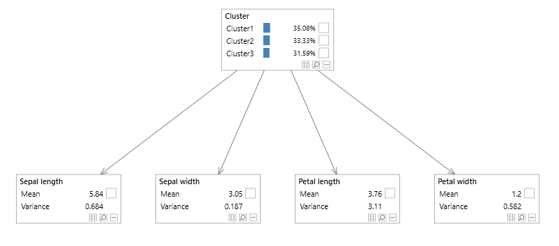
Figure 13 - Diagonal iris Mixture model
Evidence
A further advantage of this representation is that we do not lose the distinction of a variable, and therefore we can apply evidence to each variable individually within a node that contains multiple variables. In fact, some variables can have missing data, and we can still incorporate soft/virtual evidence on individual variables.
Decomposition
Bayesian networks with MVN nodes can be fully decomposed into their single variable node equivalents. We do not need to decompose an MVN network to perform inference, however it is useful to examine the equivalent SVN network.
MVN Inference
Inference in MVN Bayesian networks is largely the same as for SVN networks, however there are a number of important differences.
- We can query a node, a group of nodes, a variable, or more than one variable which may span multiple nodes
- Evidence can be applied at the granularity of a variable, so a node may be partially instantiated if some variables have missing data.
Conclusion
This article has outlined the major advantages of MVN networks, which are performance gains, graphical simplicity and an alternative parameterization.
In practice they become an indispensable tool, particularly when building models of multivariate continuous data, using techniques (or extensions of them) such
as Hidden Markov Models, Kalman filters and Vector Auto Regressive models.