Bayesian networks - an introduction
This article provides a general introduction to Bayesian networks. For the online app with sample networks and information about our software please see the following:
What are Bayesian networks?
Bayesian networks are a type of Probabilistic Graphical Model that can be used to build models from data and/or expert opinion.
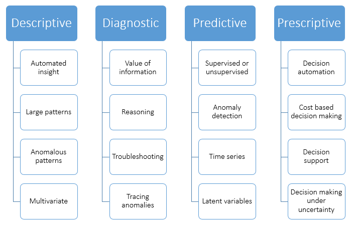
They can be used for a wide range of tasks including prediction, anomaly detection, diagnostics, automated insight, reasoning, time series prediction and decision making under uncertainty. Figure 1 below shows these capabilities in terms of the four major analytics disciplines, Descriptive analytics, Diagnostic analytics, Predictive analytics and Prescriptive analytics.
 {itemprop=image}
Figure 1 - Descriptive, diagnostic, predictive & prescriptive analytics with Bayesian networks
NOTE
They are also commonly referred to as Bayes nets, Belief networks and sometimes Causal networks.
Probabilistic
Bayesian networks are probabilistic because they are built from probability distributions and also use the laws of probability for prediction and anomaly detection, for reasoning and diagnostics, decision making under uncertainty and time series prediction.
Graphical
Bayesian networks can be depicted graphically as shown in Figure 2, which shows the well known Asia network. Although visualizing the structure of a Bayesian network is optional, it is a great way to understand a model.
 Figure 2 - A simple Bayesian network, known as the Asia network.
A Bayesian network is a graph which is made up of Nodes and directed Links between them.
Nodes
In many Bayesian networks, each node represents a Variable such as someone's height, age or gender. A variable might be discrete, such as Gender = {Female, Male} or might be continuous such as someone's age.
In Bayes Server each node can contain multiple variables. We call nodes with more than one variable multi-variable nodes.
The nodes and links form the structure of the Bayesian network, and we call this the structural specification.
Bayes Server supports both discrete and continuous variables.
Discrete
A discrete variable is one with a set of mutually exclusive states such as Gender = {Female, Male}.
Continuous
Bayes Server support continuous variables with Conditional Linear Gaussian distributions (CLG). This simply means that continuous distributions can depend on each other (are multivariate) and can also depend on one or more discrete variables.
NOTE
Although Gaussians may seem restrictive at first, in fact CLG distributions can model complex non-linear (even hierarchical) relationships in data. Bayes Server also supports Latent variables which can model hidden relationships (automatic feature extraction, similar to hidden layers in a Deep neural network).
 Figure 3 - A simple Bayesian network with both discrete and continuous variables, known as the Waste network.
Links
Links are added between nodes to indicate that one node directly influences the other. When a link does not exist between two nodes, this does not mean that they are completely independent, as they may be connected via other nodes. They may however become dependent or independent depending on the evidence that is set on other nodes.
NOTE
Although links in a Bayesian network are directed, information can flow both ways (according to strict rules described later).
Structural learning
Bayes Server include a Structural learning algorithm for Bayesian networks, which can automatically determine the required links from data.
NOTE
Note that structural learning is often not required, as there are many well known structures that can solve many problems.
Feature selection
Bayes Server supports a Feature selection algorithm which can help determine which variables are most likely to influence another. This can be helpful when determining the structure of a model.
NOTE
Another useful technique is to make use of Latent variables to automatically extract features as part of the model.
Directed Acyclic Graph (DAG)
A Bayesian network is a type of graph called a Directed Acyclic Graph or DAG. A Dag is a graph with directed links and one which contains no directed cycles.
Directed cycles
A directed cycle in a graph is a path starting and ending at the same node where the path taken can only be along the direction of links.
Notation
At this point it is useful to introduce some simple mathematical notation for variables and probability distributions.
Variables are represented with upper-case letters (A,B,C) and their values with lower-case letters (a,b,c). If A = a we say that A has been instantiated.
A set of variables is denoted by a bold upper-case letter (X), and a particular instantiation by a bold lower-case letter (x). For example if X represents the variables A,B,C then x is the instantiation a,b,c. The number of variables in X is denoted |X|. The number of possible states of a discrete variable A is denoted |A|.
The notation pa(X) is used to refer to the parents of X in a graph. For example in Figure 2, pa(Dyspnea) = (Tuberculosis or Cancer, Has Bronchitis).
We use P(A) to denote the probability of A.
We use P(A,B) to denote the joint probability of A and B.
We use P(A | B) to denote the conditional probability of A given B.
Probability
P(A) is used to denote the probability of A. For example if A is discrete with states {True, False} then P(A) might equal [0.2, 0.8]. I.e. 20% chance of being True, 80% chance of being False.
Joint probability
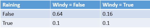
A joint probability refers to the probability of more than one variable occurring together, such as the probability of A and B, denoted P(A,B).
An example joint probability distribution for variables Raining ad Windy is shown below. For example, the probability of it being windy and not raining is 0.16 (or 16%).
NOTE
For discrete variables, the joint probability entries sum to one.
NOTE
If two variables are independent (i.e. unrelated) then P(A,B) = P(A)P(B).
Conditional probability
Conditional probability is the probability of a variable (or set of variables) given another variable (or set of variables), denoted P(A|B).
For example, the probability of Windy being True, given that Raining is True might equal 50%.
This would be denoted P(Windy = True | Raining = True) = 50%.
Marginal probability
A marginal probability is a distribution formed by calculating the subset of a larger probability distribution.
If we have a joint distribution P(Raining, Windy) and someone asks us what is the probability of it raining, we need P(Raining), not P(Raining, Windy). In order to calculate P(Raining), we can simply sum up all the values for Raining = False, and Raining = True, as shown below.
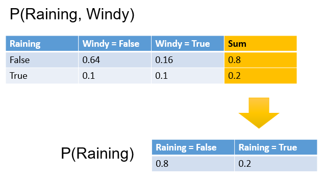
This process is called marginalization.
NOTE
When we query a node in a Bayesian network, the result is often referred to as the marginal.
NOTE
For discrete variables we sum, whereas for continuous variables we integrate.
NOTE
The term marginal is thought to have arisen because joint probability tables written in ledgers were summed along rows or columns, and the result written in the margins of the ledger.
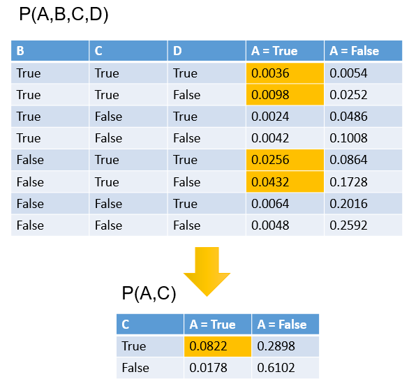
A more complicated example involving the marginalization of more than one variable is shown below.
Distributions
Once the structure has been defined (i.e. nodes and links), a Bayesian network requires a probability distribution to be assigned to each node.
NOTE
Note that it is a bit more complicated for time series nodes and noisy nodes as they typically require multiple distributions.
Each node X in a Bayesian network requires a probability distribution P(X | pa(X)).
NOTE
Note that if a node X has no parents pa(X) is empty, and the required distribution is just P(X) sometimes referred to as the prior.
This is the probability of itself given its parent nodes. So for example, in figure 2, the node Dyspnea has two parents (Tuberculosis or Cancer, Has Bronchitis), and therefore requires the probability distribution P ( Dyspnea | Tuberculosis or Cancer, Has Bronchitis ) an example of which is shown in table 1. This type of probability distribution is known as a conditional probability distribution, and for discrete variables, each row will sum to 1.
The direction of a link in a Bayesian network alone, does not restrict the flow of information from one node to another or back again, however does change the probability distributions required, since as described above, a node's distribution is conditional on its parents.
| Has Bronchitis | Tuberculosis or Cancer | Dyspnea = True | Dyspnea = False |
|---|---|---|---|
| True | True | 0.9 | 0.1 |
| True | False | 0.8 | 0.2 |
| False | True | 0.7 | 0.3 |
| False | False | 0.1 | 0.9 |
Table 1 - P ( Dyspnea | Tuberculosis or Cancer, Has Bronchitis )
Distributions in a Bayesian network can be learned from data, or specified manually using expert opinion.
Parameter learning
There are a number of ways to determine the required distributions.
- Learn them from data
- Manually specify (elicit) them using experts.
- A mixture of both.
Bayes Server includes an extremely flexible Parameter learning algorithm. Features include:
- Missing data fully supported
- Support for both discrete and continuous latent variables
- Records can be weighted (e.g. 1000, or 0.2)
- Some nodes can be learned whilst other are not
- Priors are supported
- Multithreaded and/or distributed learning.
Please see the parameter learning help topic for more information.
Online learning
Online learning (also known as adaptation) with Bayesian networks, enables the user or API developer to update the distributions in a Bayesian network each record at a time. This uses a fully Bayesian approach.
NOTE
Often a batch learning approach is used on historical data periodically, and an online algorithm is used to keep the model up to date in between batch learning.
For more information see Online learning.
Evidence
Things that we know (evidence) can be set on each node/variable in a Bayesian network. For example, if we know that someone is a Smoker, we can set the state of the Smoker node to True. Similarly, if a network contained continuous variables, we could set evidence such as Age = 37.5.
We use e to denote evidence set on one or more variables.
When evidence is set on a probability distribution we can reduce the number of variables in the distribution, as certain variables then have known values and hence are no longer variables. This process is termed Instantiation.
Bayes Server also supports a number of other techniques related to evidence:
Instantiation
The figure below shows an example of instantiating a variable in a discrete probability distribution.
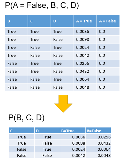
NOTE
Note that we can if necessary instantiate more than one variable at once, e.g. P(A=False, B=False, C, D) => P(C, D).
NOTE
Note that when a probability distribution is instantiated, it is no longer strictly a probability distribution, and is therefore often referred to as a likelihood denoted with the Greek symbol phi Φ.
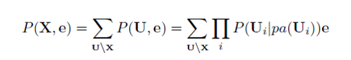
Joint probability of a Bayesian network
If U = {A1,...,An} is the universe of variables (all the variables) in a Bayesian network, and pa(Ai) are the parents of Ai then the joint probability distribution P(U) is the simply the product of all the probability distributions (prior and conditional) in the network, as shown in the equation below.
NOTE
This equation is known as the chain rule.
From the joint distribution over U we can in turn calculate any query we are interested in (with or without evidence set).
For example if U contains variables {A,B,C,D,E} we can calculate any of the following:
- P(A) or P(B), etc...
- P(A,B)
- P(A|B)
- P(A,B|C,D)
- P(A | C=False)
- ...
The problem is that joint probability distribution, particularly over discrete variables, can be very large.
Consider a network with 30 binary discrete variables. Binary simply means a variable has 2 states (e.g. True & False). The joint probability would require 230 entries which is a very large number. This would not only require large amounts of memory but also queries would be slow.
NOTE
Bayesian networks are a factorized representation of the full joint. (This just means that many of the values in the full joint can be computed from smaller distributions). This property used in conjunction with the distributive law enable Bayesian networks to query networks with thousands of nodes.
Distributive law
The Distributive law simply means that if we want to marginalize out the variable A we can perform the calculations on the subset of distributions that contain A
NOTE
The distributive law has far reaching implications for the efficient querying of Bayesian networks, and underpins much of their power.
Bayes Theorem
From the axioms of probability it is easy to derive Bayes Theorem as follows:
P(A,B) = P(A|B)P(B) = P(B|A)P(A) => P(A|B) = P(B|A)P(A) / P(B)
Bayes theorem allows us to update our belief in a distribution Q (over one or more variables), in the light of new evidence e. P(Q|e) = P(e|Q)P(Q) / P(e)
The term P(Q) is called the prior or marginal probability of Q, and P(Q|e)is called the posterior probability of Q.
The term P(e) is the Probability of Evidence, and is simply a normalization factor so that the resulting probability sums to 1. The term P(e|Q) is sometimes called the likelihood of Q given e, denoted L(Q|e). This is because, given that we know e, P(e|Q) is a measure of how likely it is that Q caused the evidence.
Are Bayesian networks Bayesian?
Yes and no. They do make use of Bayes Theorem during inference, and typically use priors during batch parameter learning. However they do not typically use a full Bayesian treatment in the Bayesian statistical sense (i.e. hyper parameters and learning case by case).
The matter is further confused, as Bayesian networks typically DO use a full Bayesian approach for Online learning.
Inference
Inference is the process of calculating a probability distribution of interest e.g. P(A | B=True), or P(A,B|C, D=True). The terms inference and queries are used interchangeably. The following terms are all forms of inference will slightly difference semantics.
- Prediction - focused around inferring outputs from inputs.
- Diagnostics - inferring inputs from outputs.
- Supervised anomaly detection - essentially the same as prediction
- Unsupervised anomaly detection - inference is used to calculate the P(e) or more commonly log(P(e)).
- Decision making under uncertainty - optimization and inference combined. See Decision graphs for more information.
A few examples of inference in practice:
- Given a number of symptoms, which diseases are most likely?
- How likely is it that a component will fail, given the current state of the system?
- Given recent behavior of 2 stocks, how will they behave together for the next 5 time steps?
NOTE
Importantly Bayesian networks handle missing data during inference (and also learning), in a sound probabilistic manner.
Exact inference
Exact inference is the term used when inference is performed exactly (subject to standard numerical rounding errors).
Exact inference is applicable to a large range of problems, but may not be possible when combinations/paths get large.
NOTE
Is is often possible to refactor a Bayesian network before resorting to approximate inference, or use a hybrid approach.
Approximate inference
- Wider class of problems
- Deterministic / non deterministic
- No guarantee of correct answer
Algorithms
There are a large number of exact and approximate inference algorithms for Bayesian networks.
Bayes Server supports both exact and approximate inference with Bayesian networks, Dynamic Bayesian networks and
Decision Graphs. Bayes Server algorithms.
NOTE
Bayes Server exact algorithms have undergone over a decade of research to make them: * Very fast * Numerically stable * Memory efficient
NOTE
We estimate that it has taken over 100 algorithms/code optimizations to make this happen!
Queries
As well as complex queries such as P(A|B), P(A, B | C, D), Bayes Server also supports the following:
- Log-likelihood
- Most probable explanation
- Conflict
- Comparison query to compare scenarios.
Analysis
Bayes Server also includes a number of analysis techniques that make use of the powerful inference engines, in order to extract automated insight, perform diagnostics, and to analyze and tune the parameters of the Bayesian network.
Dynamic Bayesian networks
Dynamic Bayesian networks (DBNs) are used for modeling times series and sequences. They extend the concept of standard Bayesian networks with time. In Bayes Server, time has been a native part of the platform from day 1, so you can even construct probability distributions such as P(X[t=0], X[t+5], Y | Z[t=2]) (where t is time).
For more information please see the Dynamic Bayesian network help topic.
Decision graphs
Once you have built a model, often the next step is to make a decision based on that model. In order to make those decisions, costs are often involved. The problem with doing this manually is that there can be many different decisions to make, costs to trade off against each other, and all this in an uncertain environment (i.e. we are not sure of certain states).
Decision Graphs are an extension to Bayesian networks which handle decision making under uncertainty.
For more information please see the Decision Graphs help topic.