Decision graphs
Introduction
Decision Graphs, also known as Influence Diagrams, extend Bayesian networks with the concepts of Utilities (e.g. profits/loses/gains/costs) and Decisions. This facilitates decision making under uncertainty, also known as Decision automation.
Note that you can also use Evidence optimization to minimize/maximize/goal-seek a function/continuous variable/discrete state.
This article provides technical detail about decision graphs. For a higher level discussion please see the Introduction to Decision automation.
The objective of a Decision Graph is to find an optimal strategy (set of decisions) which maximizes the overall utility (e.g. profit/loss) of the network.
This allows us to make cost based decisions based on models learned from data and/or built from expert opinion.
Utilities
One or more Utility variables can be added to a Bayesian network, allowing the encoding of values which are typically positive to represent a gain/profit or negative to represent a loss or cost. These values are called utilities.
Like a standard continuous probability/chance node a Utility node also has a distribution associated with it. As is the case for probability/chance nodes this distribution is conditional on its parents. For example, a utility node U1 with parents C1 and D2 would have a distribution P(U1 | C1, D2).
This distribution can have variances associated with each utility or the variance can be fixed to zero.
Bayes Server allows both discrete and continuous probability/chance nodes to co-exist with utility and decision nodes.
When a network contains multiple utility nodes, a leaf utility must be added. This forms an overall utility for the network, by weighting its parents. The reason we require this leaf utility is two-fold. First it allows the utility to be queried just like a standard continuous variable, in fact you can perform joint queries also. Second it allows you to weight parent utilities.
Decisions
One or more Decision variables can also be added to a Bayesian network. Each decision variable is a discrete variable whose states represent actions/decisions that can be made.
Policy
Like a standard discrete probability/chance node a Decision node also has a distribution associated with it. As is the case for probability/chance nodes this distribution is conditional on its parents. For example, a decision node D1 with parents C1 and D2 would have a distribution P(D1 | C1, D2).
The distribution associated with a decision node is called a policy and encodes the decision to take in each parent combination (scenario).
Policies can either be learned from data, or specified manually. When specified manually they are typically initially set to a uniform distribution.
Strategy
All the policies for each decision node taken together form what is called a strategy. The purpose therefore, of a decision graph, is to find a strategy (set of decisions) which maximizes the utility of the network.
LIMIDS
Bayes Server supports a particular class of Decision graphs (influence diagrams) called Limited Memory Influence Diagrams (LIMIDS).
These do not impose a specific ordering on the decisions, and are therefore more powerful than some simpler types of Decision Graph.
Inference
Inference in Decision graphs is the process of attempting to find the strategy which maximizes the utility of the network. With LIMIDS this requires an iterative optimization routine.
The inference algorithm starts with the given policies for each decision node, and any evidence set. It will then iteratively try new policies until a local maximum utility is found.
Note that the algorithm will not overwrite the initial policies specified in the network (found either manually or through parameter learning).
Queries
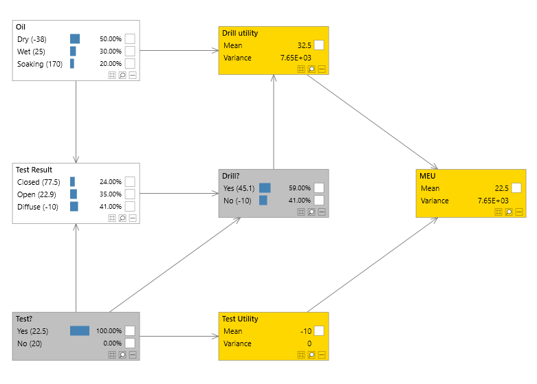
You will notice in the Bayes Server User Interface that utility values will appear next to each discrete state or action in the network. This is performed automatically when queries are added and a utility node is found in the network. For example, if a network contains a discrete chance node P1, and the leaf utility node U1, instead of the query P(P1) that is normally calculated, the network calculated P(P1, U1) and displays the values of U1 along side each state in P1.
To retrieve the locally optimal policies found by the inference engine you can query each decision node given its parents.
Joint queries can be performed in the normal way. Joint queries can include one or more utility variables, continuous and discrete chance variables and decision variables.
Cost/profit surfaces
Since Bayes Server allows utility variables to be included in queries in the normal way, and they can co-exist in queries with other chance/probability nodes and other utilities or decisions, we can generate data which could be used to plot a 3D cost/profit surface.
Bayes Server allows utility variables to be combined with both continuous and discrete chance nodes as well as other utilities and decisions. This allows us to build complex multi-dimensional cost/profit models. The chance/probability nodes can even be latent/hidden as found in mixture models (feature engineering).
Consider a model with a discrete chance node P1, continuous chance nodes X and Y, a utility node U1, and one or more decision nodes. We can use the inference algorithm to query P(U1, X, Y | P1)
Evidence on decision variables
Decision variables behave in a different way to chance/probability variables when evidence is set on them (a decision is made). This is due to the fact that making a decision is an external user making a decision as opposed to an observation being made.
Parameter learning
You can train the distributions in a decision graph in the normal way. Utility distributions will reflect the variances in your cost/profit data and initial policies will be learned for the distributions of decision nodes, which will then be the initial policies used during the inference/optimization procedure described above.