Introduction to probability
In this article we introduce some basic concepts in probability.
Variables
A variable refers to a value that can change between measurements/examples such as quantity or state. This could be a discrete variable such as Risk with possible values {Red, Amber, Green} or a continuous variable such as Age (e.g. 22 or 37 or 65).
The symbols X, Y & Z are typically used when we are concerned with general rules (theorems) involving variables.
Discrete Variables
Discrete variables can take on one of a set of distinct states. For example, the variable Risk might have possible states {Red, Amber, Green} meaning that each measurement/example would either be Red, Amber or Green.
The set of states in a variable must be exhaustive, simply meaning that the states cover all possible scenarios. They are also mutually exclusive, meaning that you cannot be in more that one state at the same time.
It is important to point out that although the actual (known) value of a discrete variable can only be one of the mutually exclusive states, if we do not know the exact state of a variable, we can still assign a certainty of being in each state. For example {Red = 30%, Amber = 60%, Green = 10%}.
If the states are not mutually exclusive, e.g. a person plays both football and tennis, then we need more than one variable, e.g. Football {True, False} and Tennis {True, False}.
Continuous variables
A continuous variable can be assigned a value which is a real number. For example, the value of a variable Speed could be 0 kph, 25.5 kph, 100 kph etc...
Again it is important to point out that if we do not know the exact value of a continuous variable we can still assign a certainty to it lying within a range of values. E.g. we are 30% sure that the car was traveling at at least 70 kph.
Discretization
It is sometimes useful to convert a continuous variable to a discrete variable. For example, some algorithms do not support continuous variables.
This can be done by creating bins which represent a range of values. Each bin then becomes a discrete state of a derived discrete variable.
There are a number of different algorithms commonly used to determine the bins (ranges). For example, equal ranges (each range has the same size), equal frequencies (each bin has the same number of records) or clustering (a machine learning algorithm is employed).
Columns of data
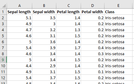
Usually a variable corresponds 1-to-1 with a column of data in a spreadsheet or database. For example, the variables in the Microsoft Excel spread-sheet shown below are as follows:
| Variable | Value Type |
|---|---|
| Sepal length | Continuous |
| Sepal width | Continuous |
| Petal length | Continuous |
| Petal width | Continuous |
| Class | Discrete |
Probability
A probability is quantified as a number between 0 and 1. It tells us how likely a particular situation is, such as a discrete variable being in a particular state, or a continuous variable being within a range of values. A value of 0 indicates no chance (impossible) and a value of 1 is a sure thing (certainty).
For example, the probability of Country=US might equal 0.1, meaning that we think that there is a 10% chance a person lives in the US. In mathematical notations this is written P(Country=US) = 0.1, or where the context of the state 'US' is clear you might see it written as P(US) = 0.1.
Joint probability
A probability may be based on more than one variable. For example, the probability of Rain {True, False} and Wind {True, False} both being True might be 0.1 (10%). In math notation this would be written as P(Raining=True, Windy=True). This type of probability also has a special name called a Joint probability.
Conditional probability
A probability value can be conditioned on other variables. For example we may require the probability of Raining being True given that we know Windy is True. In mathematical notation this would be written P(Raining=True | Windy=True).
Multiple states / ranges
You can also have a probability which is based on multiple states or ranges (over one or more variables). For example if the variable Hair Length has states {Short, Medium, Long} we might be interested in the probability that someone does not have short hair.
Probability vs probability distribution
We will cover probability distributions later in the article, but it is useful to explain what the difference is at this point.
A probability refers to the number between 0 and 1 which tells us how likely a particular situation is, for example P(Country=US)=0.1.
A probability distribution on the other hand, provides us with a way of getting the probability value for each possible outcome.
The probability distribution for a variable Country therefore provides us with the probability for country P(Country=US) as well as the probability for UK P(Country=UK), Japan P(Country=Japan) and so on.
In mathematical notation the probability distribution for Country is written P(Country). The only difference between this notation and that for each of the probability values returned from the probability distribution is that the state/outcome (US, UK, etc...) is omitted.
In mathematics a probability distribution is a type of function. i.e. a function which returns a probability for each outcome. A discrete probability distribution is often called a Probability Mass Function and a continuous distribution a Probability Density Function.
Voltaire Quote
The following famous quote from Voltaire reminds us why probability is such a useful concept.
Doubt is not a pleasant condition, but certainty is absurd.
- Voltaire
Probability distribution
A probability distribution tells us how likely each possible state/outcome (or range) is.
Probability Mass Function (pmf)
For discrete variables, a probability distribution provides us with a probability value for each state/outcome. To be a valid distribution, the sum of these values must equal 1 (since states are mutually exclusive and exhaustive).
For example, if a variable Hair Length had possible states {Short, Medium, Long}, a discrete distribution might look like [0.2, 0.3, 0.5]. This means that the probability of Hair Length = Short is 0.2 (20%), Hair Length = Medium is 0.3 (30%) and Hair Length = Long is 0.5 (50%).
A discrete probability distribution is known as a Probability Mass Function.
Bernoulli distribution
When a discrete variable has only two possible states (outcomes) such as True or False, we can use two probabilities (e.g. True=0.7, False=0.3) to define a probability distribution.
In fact since the probabilities must sum to 1, we actually only need one of these values to fully specify this distribution.
This distribution has a special name called the Bernoulli distribution.
The Bernoulli distribution, which helps us model a particular outcome, is not to be confused with the Binomial distribution which helps us model a sequence of outcomes. In fact when a Binomial distribution has only one outcome it is a Bernoulli distribution.
Multinoulli distribution
An extension of the Bernoulli distribution can be used when we have more than two outcomes. For example, we might have a variable Hair Length with possible outcomes {Short, Medium, Long} and use the distribution [0.2, 0.3, 0.5].
This distribution is often called a Multinoulli distribution. Again this is not to be confused with the Multinomial distribution which is used to model a sequence of outcomes.
Percentages
Non-mathematicians tend to talk about probabilities in terms of percentages rather than a number between 0 and 1.
A discrete probability can be multiplied by 100 to give its percentage equivalent. For example a probability of 0.25 is equivalent to a 25% chance.
Note that this is consistent with Microsoft Excel. In Excel, 0.2 is equivalent to 20%. If you multiply either by 100 you get 20. Also if you enter 0.2 in a cell and format the cell with the percentage button it will display 20%.
Probability density function (pdf)
For continuous variables a probability distribution tells us what the chance of being within a range of values is.
Whereas a discrete probability distribution must sum to one, the analogous for a continuous probability distribution is that the integral must sum to 1. (E.g. for a single variable, the area under the curve must sum to 1).
In many cases you can think of summing as being equivalent to integrating, when dealing with discrete or continuous distributions respectively.
Note that for continuous variables, the chance of having an individual value tends to zero, as there are infinitely many possible real number values the variable can take.
Gaussian distribution
A very common example of a continuous distribution is the Gaussian (Normal) probability distribution.
This is a distribution from the exponential family of distributions (it has an e term in the equation).
Cumulative density function (cdf)
For continuous variables the cumulative density function tells us what the chance of being less than or equal to a particular value is.
As you might expect, the cdf evaluated at x, is simply the the area under the probability density function from minus infinity to x
Joint probability distribution
Earlier we introduced the Joint probability, for example P(Raining=True, Windy=True). A joint probability distribution gives us the joint probability value for each possible combination of states (outcomes) from both variables.
For example, the joint distribution over Raining and Windy would be able to return the probability value for each possible combination:
| Raining | Windy | Probability |
|---|---|---|
| True | True | 0.10 |
| True | False | 0.15 |
| False | True | 0.25 |
| False | False | 0.5 |
Note that the sum (or integral) of a joint probability distribution is always 1.
The mathematical notation for this joint probability distribution is P(Raining, Windy).
In set notation you will often see this written as P(Raining ∩ Windy), however in this article we will not use this form.
Conditional probability distribution
Earlier we introduced the Conditional probability, e.g. P(Raining=True | Windy=True).
A conditional probability distribution gives us the conditional probability value for each possible combination of states (outcomes) from both variables.
For example, the conditional distribution over Raining and Windy would be able to return the conditional probability value for each possible combination. For example:
| Raining | Windy | Probability |
|---|---|---|
| True | True | 0.286 |
| True | False | 0.231 |
| False | True | 0.714 |
| False | False | 0.769 |
The mathematical notation for this conditional probability distribution is P(Raining | Windy).
In the expression P( X | Y ), the variable(s) X are called Head variables and Y are called Tail variables.
The sum of a conditional probability distribution is always 1 for each Tail combination. The only Tail variable in the example above is Windy therefore the sum of probability values given that Windy=True will always equal 1, and the sum given Windy=False will be 1 also.
Axioms of probability
A number of simple rules exist called the Axioms of probability. We will describe them in simple terms, but the interested reader may wish to consult a probability text.
Given a variable S with states (outcomes) :
- and , this just means that the probability of being in each state (outcome) must have a value between 0 and 1
- or , this means that the sum of all probability values must equal 1. i.e. the states are exhaustive (cover all outcomes).
- , this means that the joint probability of states from the same variable is equal to their sum. I.e. the states are mutually exclusive. E.g. if a variable Raining can be True or False, when considering an individual record, it cannot be both raining and not raining at the same time. Note that if we do not know the actual outcome (perhaps we are in a room with no windows), we can still have a probability of being in each state, e.g. [0.3, 0.7] meaning that we are 30% sure it is raining.
Consequences
There are a number of consequences that follow directly from the axioms of probability.
One that is especially important is:
P(A,B) = P(A|B)P(B)
As we will see later, Bayes' theorem and its applications follow from this equation.
Independence
If two variables are independent (i.e. unrelated) then P(A,B) = P(A)P(B). Note that A and B could also be groups of variables.
Groups of variables are often denoted with a bold character, such as X or Y.
Independence between X and Y simply means that varying X will have no impact on Y and vice versa.
Conditional Independence
Variables A and C are independent given B, if P(A|B) = P(A|B,C).
What this means is that certain variables will become conditionally independent of each other depending on what is known about other variables (evidence), i.e. they will vary independently given certain evidence.
For example, the probability of having short hair might be independent of someone's height, given that we know someone is male.
Marginal probability distribution
A marginal probability distribution is formed by calculating the subset of a larger probability distribution. For example calculating P(X) from P(X, Y, Z) or P(X,Y) from P(X,Y,Z).
Many use the term to refer to distributions that contain only a single variable, however any subset is a valid marginal.
Consider the joint probability over the variables Raining and Windy shown below:
P(Raining, Windy)
| Raining | Windy = False | Windy = True |
|---|---|---|
| False | 0.64 | 0.16 |
| True | 0.1 | 0.1 |
If someone asks us what is the probability of it raining, we need P(Raining), not P(Raining, Windy).
In order to calculate P(Raining), we can simply sum up all the values for Raining = False, and Raining = True, as shown below.
P(Raining, Windy)
| Raining Windy = False | Windy = True | Sum |
|---|---|---|
| False | 0.64 | 0.16 |
| True | 0.1 | 0.1 |
This is known as marginalization, and the result we were after is shown below.
P(Raining)
| Raining = False | Raining = True |
|---|---|
| 0.8 | 0.2 |
For discrete variables we sum, whereas for continuous variables we integrate.
Although it is not known for sure, many believe the term marginalization came about through the use of ledgers for basic accounting. The totals (sums) would be recorded in the margins, hence the term marginalization.
Bayes Theorem
Definition
Derivation
The equation specified in Bayes' theorem can be simply derived from standard probability, as follows:
From the consequences that follow from the axioms of probability we get that P(A,B) = P(A|B)P(B) and equivalently P(A,B)=P(B|A)P(A).
Therefore P(A|B)P(B) = P(B|A)P(A) which when rearranged is
P(A|B) = P(B|A)P(A) / P(B), which is Bayes' theorem.
Sometimes Bayes' theorem is written without the denominator as P(A|B) ∝ P(B|A)P(A) where the symbol ∝ in math means is proportional to. P(B) is a normalization term, to ensure that the probability sums/integrates to 1. This form is quite common and used when the denominator has no bearing on the end computation.
Bayes' theorem can be used when we need to invert the variables we are conditioning on, such as to . For example, we may have probabilities of the form P(Symptom | Disease) and P(Disease), and we wish to calculate the P(Disease | Symptom). To do this we could use Bayes' Theorem.
Bayesian statistics
In Bayesian statistics, Bayes' theorem can be used used to incrementally update a model M from data D.
This can be done using Bayes Theorem as follows:
Each term in this equation has a name. P(M|D) is called the Posterior, P(D|M) the likelihood, P(M) the Prior, and P(D) the Marginal likelihood or Probability of Evidence.
The term likelihood can easily be confusing, as in some fields the term likelihood is used to refer to the marginal likelihood. To avoid confusion you could choose to use marginal likelihood for P(D) and conditional likelihood for P(M|D).
At some points in history, Bayesian statistics has been considered controversial. This was due to the subjective nature of the choice of prior P(M). However Bayesian statistics is now mainstream, and if anything the balance may have swung the other way, with many advocating its use while questioning frequentist techniques such as p-values. Whatever your stance, Bayes' Theorem is useful in both frequentist and Bayesian statistics.
Priors
Priors are used to give an initial starting point from which we can learn. For example, if a cricketer scores 200 runs in their first test match, would we predict that they would score 200 in their second? A Bayesian approach would start with an initial model (prior), perhaps based on batting averages given the characteristics of the player, and the prediction would be based on both the prior and the first score.
As more data is acquired the frequentist and Bayesian approaches converge to the same result.
Conceptually priors can be though of as virtual data. A bit like inserting a few records at the beginning of our data. These virtual records could be based on similar historical results or if we do not have historical data we may use our judgement.
There are a number of common priors used in practice. They are typically conjugate, simply meaning that when plugged into Bayes' theorem, the resulting distribution/model is of the same form as the original. Examples of conjugate priors are the Beta distribution (conjugate of the Bernoulli), its extension the Dirichlet distribution (conjugate of the Multinoulli) and the normal inverse Wishart (conjugate of the multi-variate Gaussian/Normal).