Hybrid Network | Manual Construction Tutorial
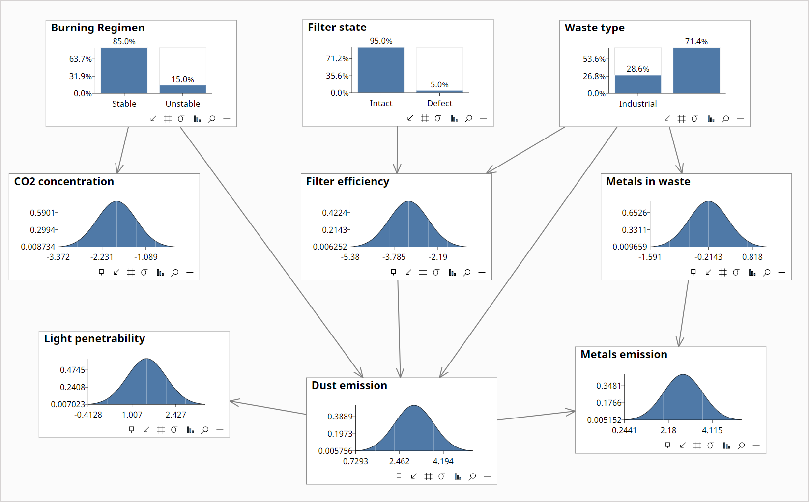
In this tutorial we will manually construct the Waste hybrid Bayesian network shown below. A hybrid network contains both Discrete and Continuous variables.
This network is also included as a sample network with Bayes Server called Waste
The steps to build the network are listed below, along with their data driven alternatives.
- Manually add nodes (alternatively we can Add nodes from data)
- Manually add links (alternatively we can use Structural Learning)
- Manually specify the node distributions (alternatively we can use Parameter learning)
You can mix and match the above steps. For example you could 1. Add nodes from data, 2. Add links manually and then 3. Learn the node distributions from data. Futhermore you could learn some node distributions from data while specifying some manually.
Create a new model
- Either click File->New from the main menu, or from the Start Page click New Empty Network.
Add Burning Regimen Node
From the Build tab on the main menu, click Node->Discrete.
Change the Name to Burning Regimen.
Ensure the node has 2 states added, and name them Stable and Unstable by double clicking on each state name.
The New Node dialog should look like this:
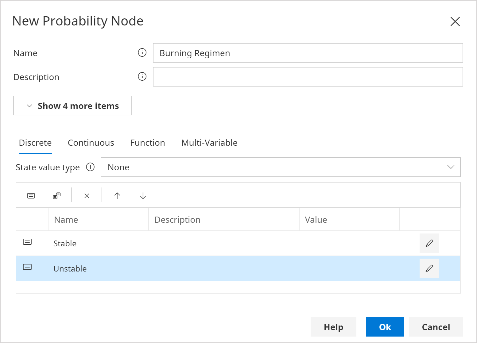
- Click Ok to add the new node.
Add additional discrete Nodes
- Repeat the previous step twice using the following node names and states instead:
- Filter state
- Intact
- Defect
- Waste type
- Industrial
- Household
- Filter state
Add CO2 concentration
From the Build tab on the main menu, click Node->Continuous.
Change the Name to CO2 concentration.
The New Node dialog should look like this:
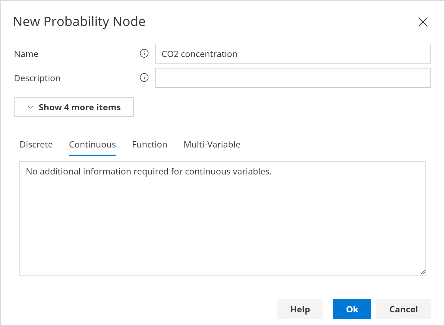
- Click Ok to add the new node.
Add additional continuous Nodes
- Repeat the previous step using the following node names instead:
- Filter efficiency
- Metals in waste
- Light penetrability
- Dust emission
- Metals emission
Position nodes
- For each node, click and drag to position similar to below:
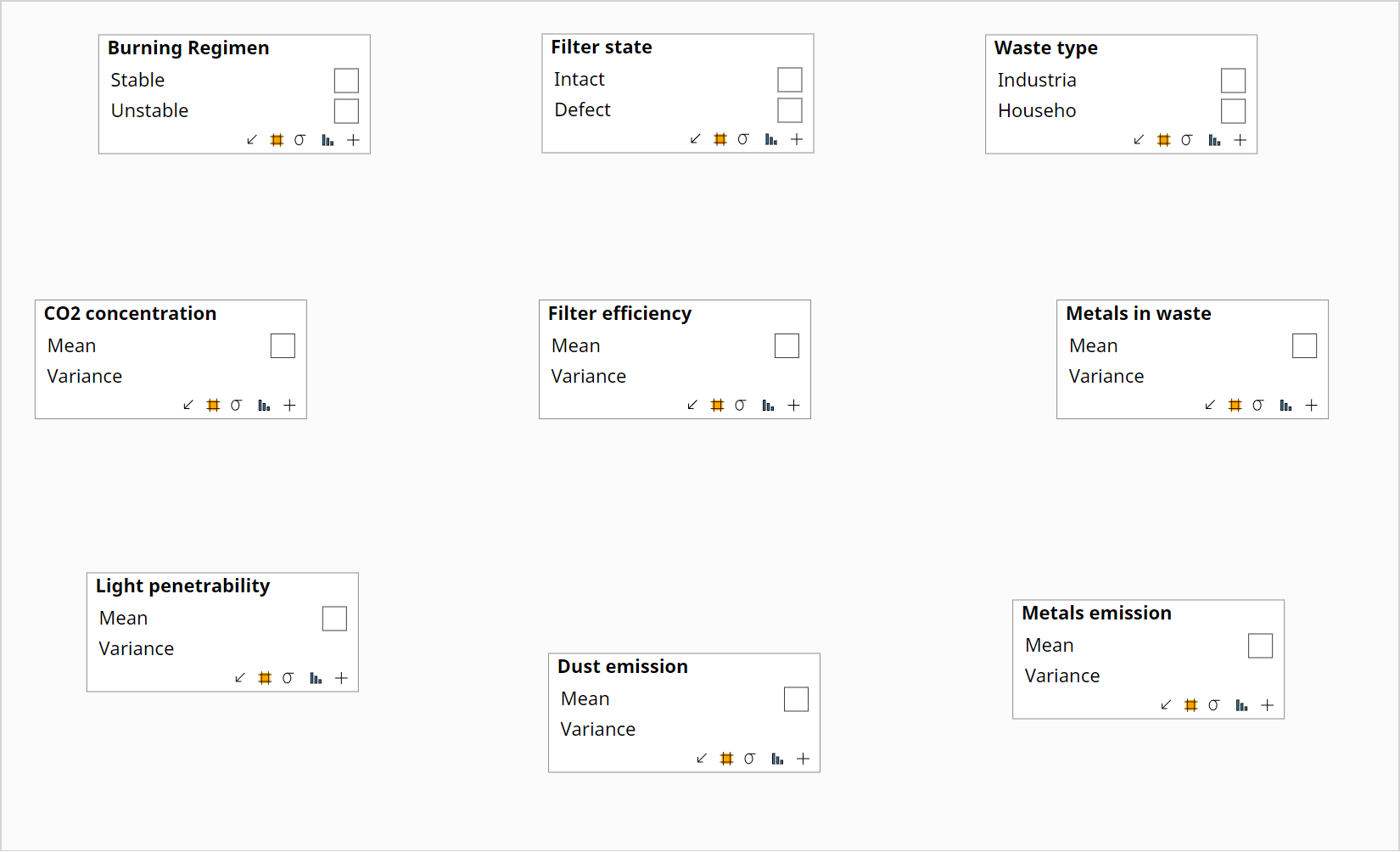
Node chart type
- From the Display tab on the main menu, click Select -> Discrete Nodes.
- From the Display tab on the main menu, click Node Chart -> Clustered Column.
- From the Display tab on the main menu, click Select -> Continuous Nodes.
- From the Display tab on the main menu, click Node Chart -> Pdf.
- To see the result of the previous action, from the Query tab, click Add -> All nodes to query the network.
- From the Display tab on the main menu, click Select -> All Nodes.
- Resize one of the nodes, by dragging the thumbnail on one corner of the node, to match the image below.
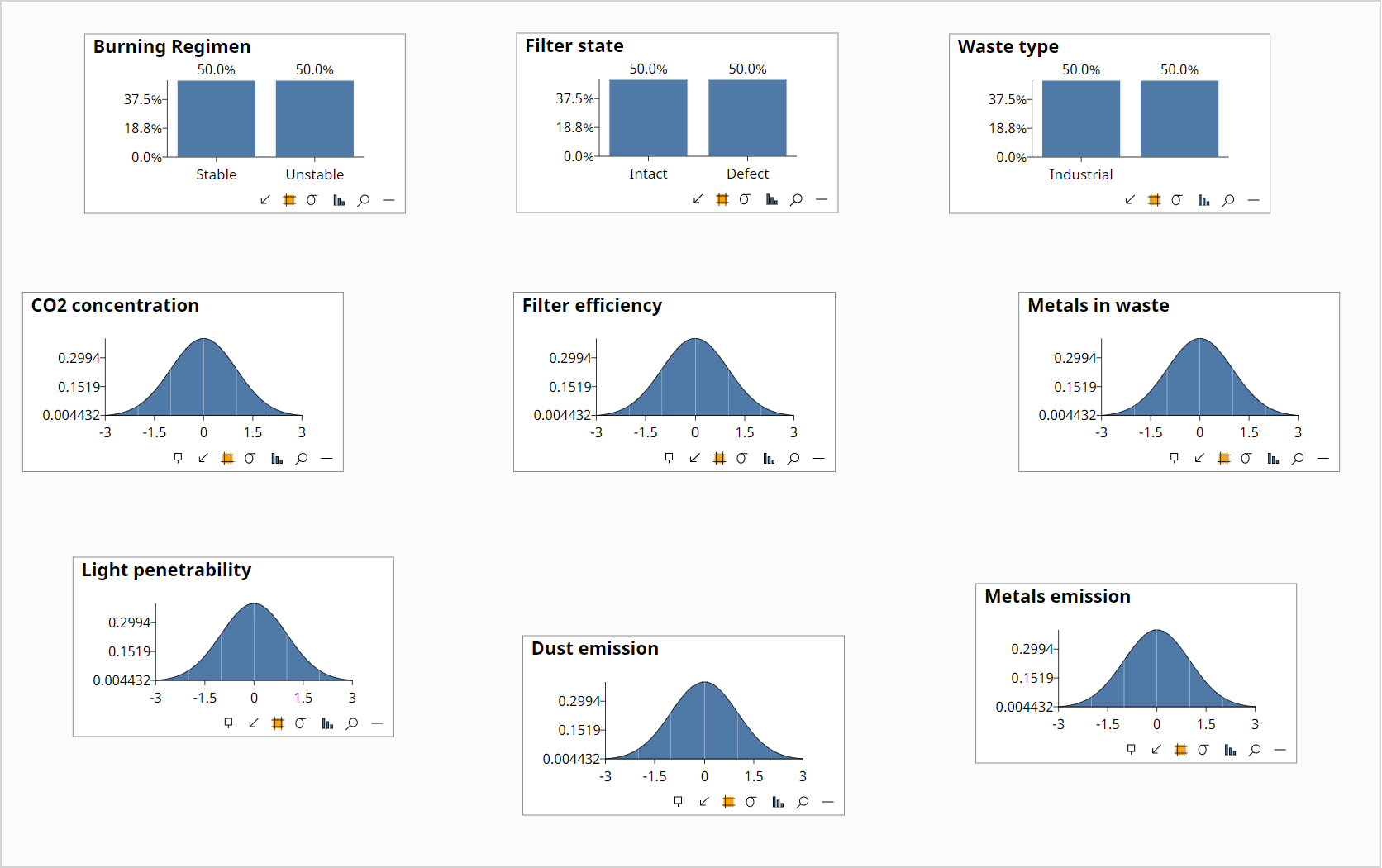
You can also select one or more nodes by holding down the Ctrl (⌘ on mac) or Shift keys when clicking nodes, or clicking in whitespace and dragging a bounding box.
Add Links
Now that the nodes have been added we can manually add some links.
- From the Build tab on the main menu, click Link -> Add link.
- Choose Burning Regimen in the From dropdown.
- Choose CO2 concentration in the To dropdown.
- Click Ok.
- Repeat for the following links
- Burning Regimen -> Dust emission
- Filter state -> Filter efficiency
- Waste type -> Filter efficiency
- Waste type -> Dust emission
- Waste type -> Metals in waste
- Filter efficiency -> Dust emission
- Metals in waste -> Metals emission
- Dust emission -> Light penetrability
- Dust emission -> Metals emission
You can select a pair of nodes before launching the New Link dialog, and this will auto-populate the From and To fields.
The network should now look like:

Define the distribution for Burning Regimen
- Click the Burning Regimen node to select it.
- From the Build tab of the main menu, click Distributions -> Edit Distribution(s).
- Click Auto-fit so the labels are easier to see.
- Double click in each cell to edit, changing the probabilities to the values in the table below.
| Burning Regimen=Stable | Burning Regimen=Unstable |
|---|---|
| 0.85 | 0.15 |
The dialog should look similar to the following:
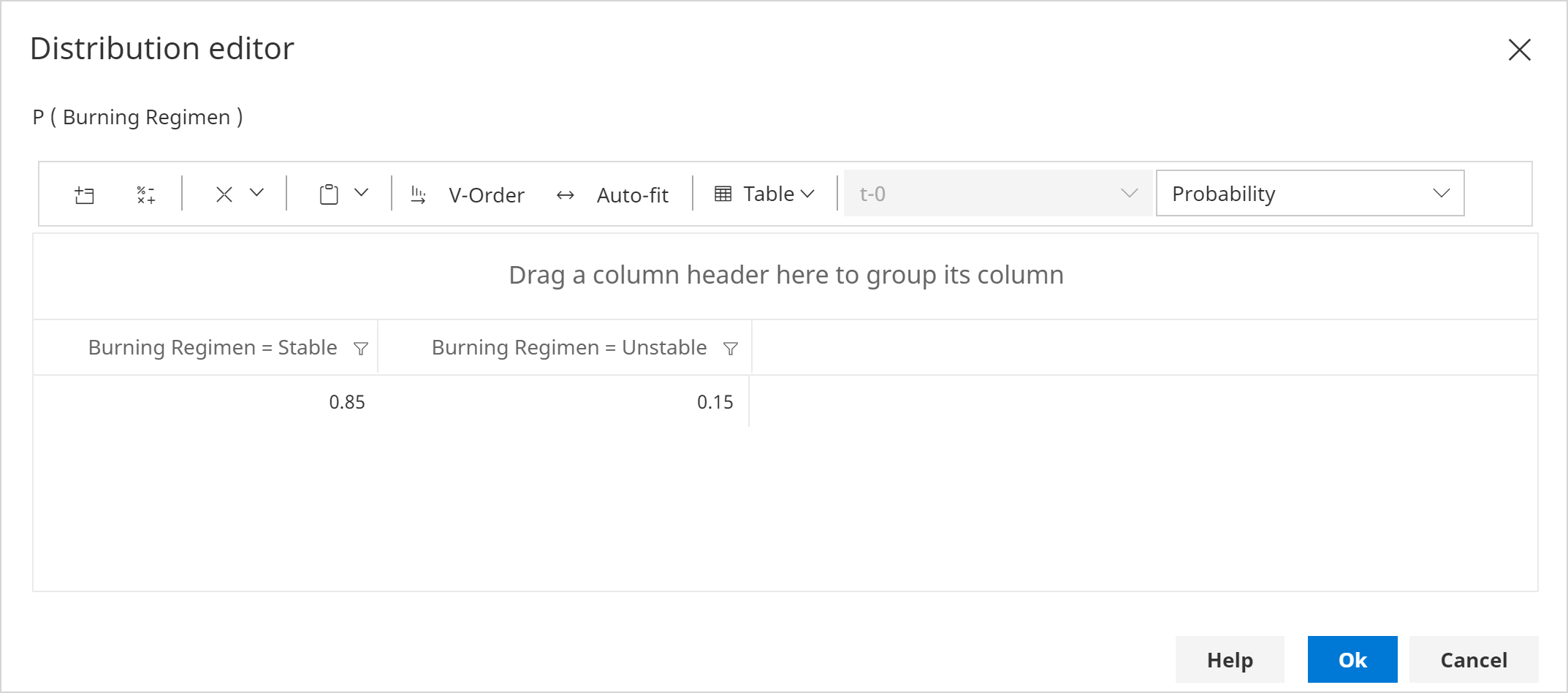
- Click OK.
Define the distribution for Filter state
- Click the Filter state node to select it.
- From the Build tab of the main menu, click Distributions -> Edit Distribution(s).
- Click Auto-fit so the labels are easier to see.
- Double click in each cell to edit, changing the probabilities to the values in the table below.
| Filter state=Intact | Filter state=Defect |
|---|---|
| 0.95 | 0.05 |
- Click OK.
Define the distribution for Waste type
- Click the Waste type node to select it.
- From the Build tab of the main menu, click Distributions -> Edit Distribution(s).
- Click Auto-fit so the labels are easier to see.
- Double click in each cell to edit, changing the probabilities to the values in the table below.
| Waste type=Industrial | Waste type=Household |
|---|---|
| 0.285714 | 0.714286 |
- Click OK.
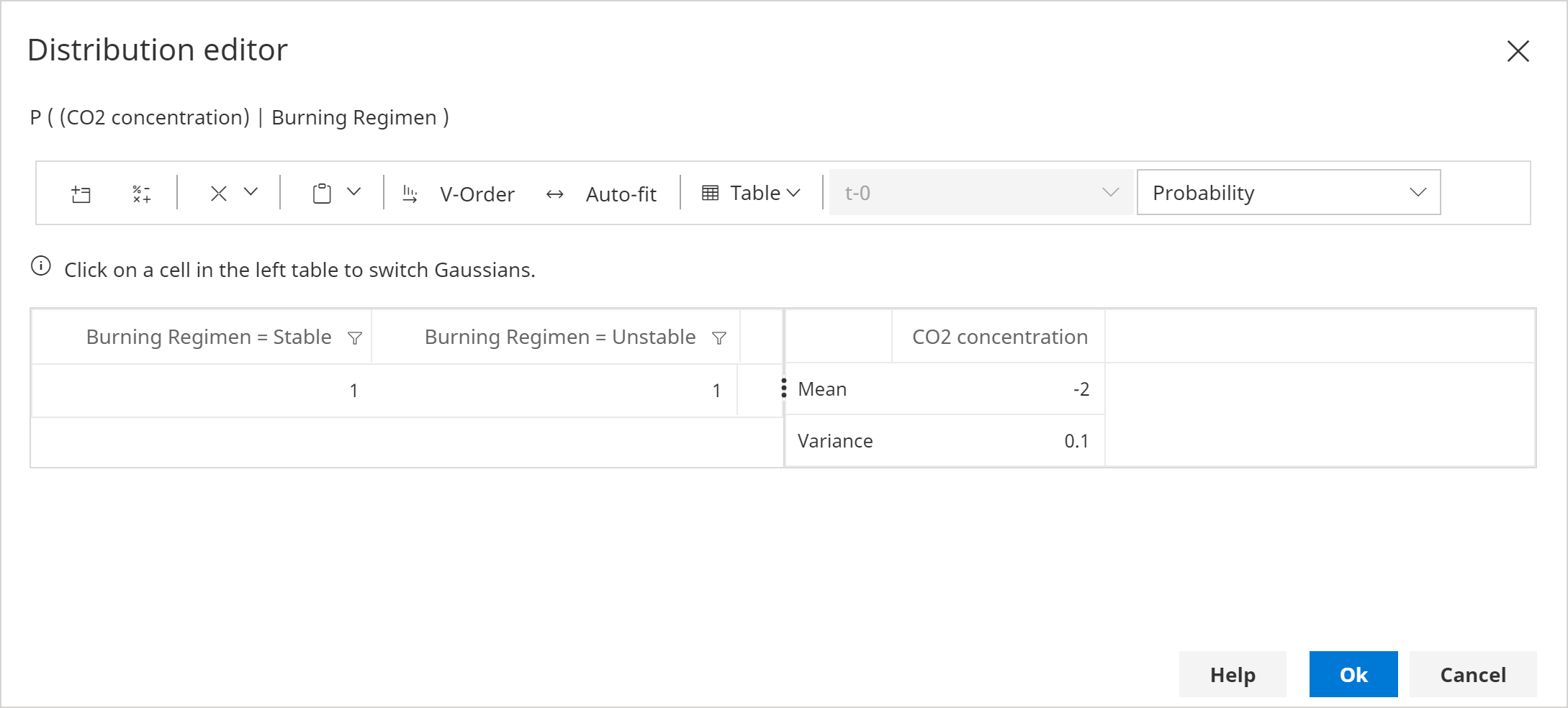
Define the distribution for CO2 concentration
Note that we must define P(CO2 concentration | Burning Regimen) which is a conditional Gaussian distribution (mixture of Gaussians).
- Click the CO2 concentration node to select it.
- From the Build tab of the main menu, click Distributions -> Edit Distribution(s).
- Click Auto-fit so the labels are easier to see.
- In the left hand pane, click on the cell containing the value 1 under Burning Regimen = Stable.
This allows us to edit the Gaussian corresponding to P(CO2 concentration | Burning Regimen = Stable)
- In the right hand pane, double click in each cell to edit, changing the values to those shown in the table below.
| CO2 concentration | |
|---|---|
| Mean | -2.0 |
| Variance | 0.1 |
The dialog should look similar to the following:
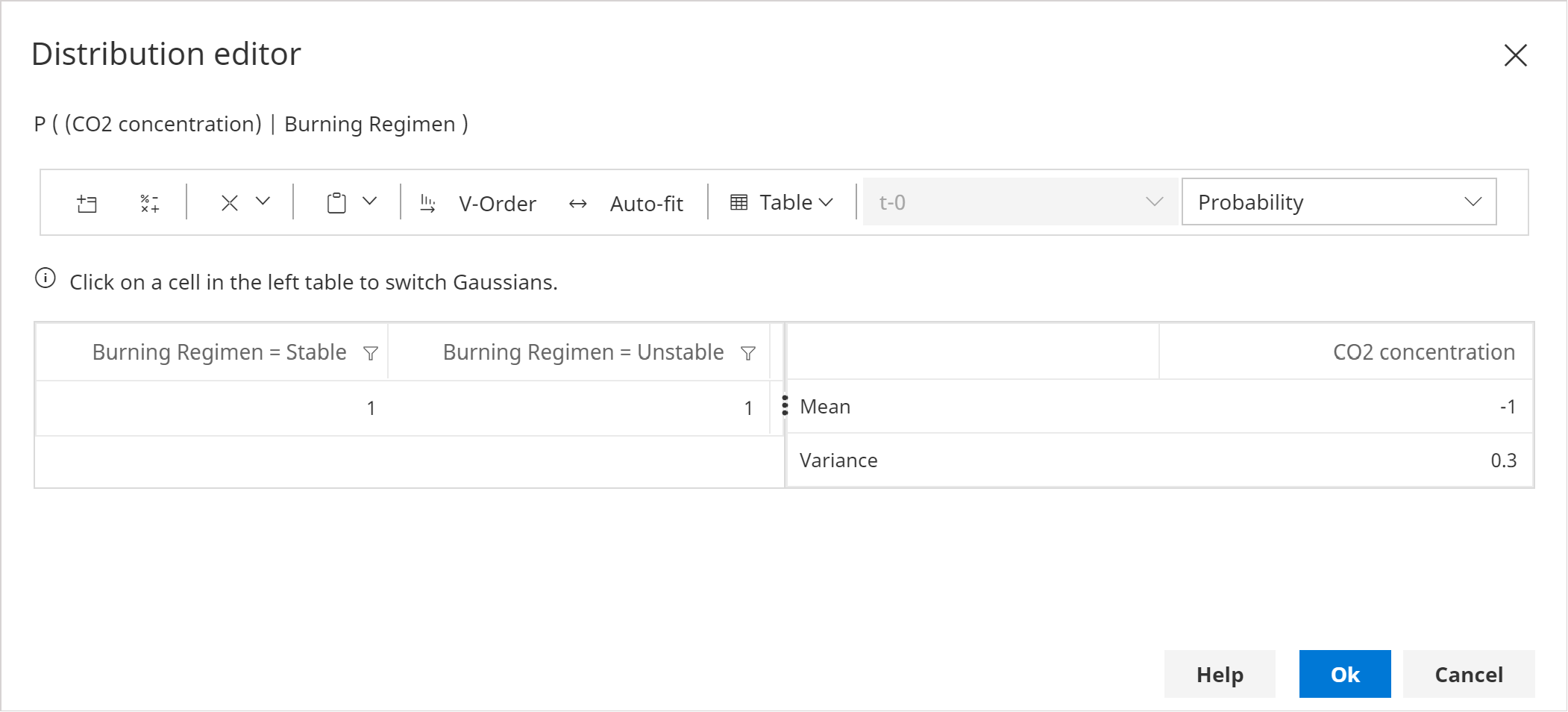
- In the left hand pane, click on the cell containing the value 1 under Burning Regimen = Unstable.
This allows us to edit the Gaussian corresponding to P(CO2 concentration | Burning Regimen = Unstable)
- In the right hand pane, double click in each cell to edit, changing the values to those shown in the table below.
| CO2 concentration | |
|---|---|
| Mean | -1.0 |
| Variance | 0.3 |
The dialog should look similar to the following:
- Click OK.
Define the distribution for Filter efficiency
Note that we must define P(Filter efficiency | Filter state, Waste type) which is a conditional Gaussian distribution (mixture of Gaussians).
- Click the Filter efficiency node to select it.
- From the Build tab of the main menu, click Distributions -> Edit Distribution(s).
- Click Auto-fit so the labels are easier to see.
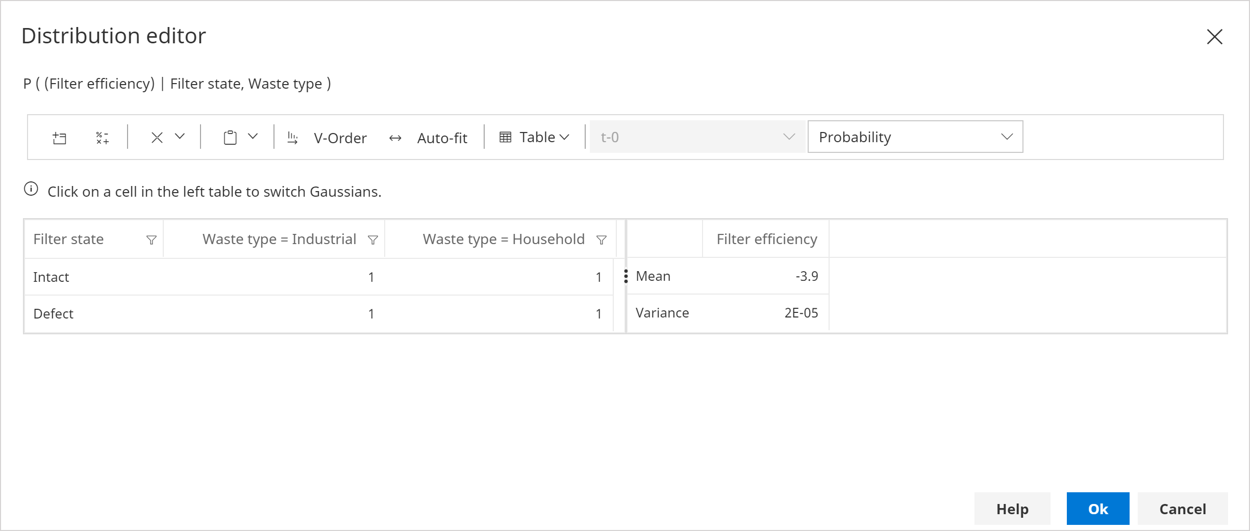
- In the left hand pane, click on the cell containing the value 1 under Filter State = Intact and Waste type = Industrial.
This allows us to edit the Gaussian corresponding to P(Filter efficiency | Filter state = Intact, Waste type = Industrial)
- In the right hand pane, double click in each cell to edit, changing the values to those shown in the table below.
| Filter efficiency | |
|---|---|
| Mean | -3.9 |
| Variance | 2e-5 |
The dialog should look similar to the following:
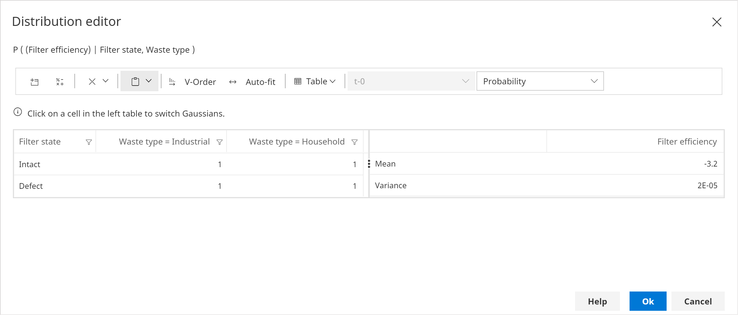
- In the left hand pane, click on the cell containing the value 1 under Filter State = Intact and Waste type = Household.
This allows us to edit the Gaussian corresponding to P(Filter efficiency | Filter state = Intact, Waste type = Household)
- In the right hand pane, double click in each cell to edit, changing the values to those shown in the table below.
| Filter efficiency | |
|---|---|
| Mean | -3.2 |
| Variance | 2e-5 |
The dialog should look similar to the following:
- In the left hand pane, click on the cell containing the value 1 under Filter State = Defect and Waste type = Industrial.
This allows us to edit the Gaussian corresponding to P(Filter efficiency | Filter state = Defect, Waste type = Industrial)
- In the right hand pane, double click in each cell to edit, changing the values to those shown in the table below.
| Filter efficiency | |
|---|---|
| Mean | -0.4 |
| Variance | 0.0001 |
- In the left hand pane, click on the cell containing the value 1 under Filter State = Defect and Waste type = Household.
- In the right hand pane, double click in each cell to edit, changing the values to those shown in the table below.
| Filter efficiency | |
|---|---|
| Mean | -0.5 |
| Variance | 0.0001 |
- Click OK
Define the distribution for Metals in waste
- Click the Metals in waste node to select it.
- From the Build tab of the main menu, click Distributions -> Edit Distribution(s).
- Click Auto-fit so the labels are easier to see.
- In the left hand pane, click on the cell containing the value 1 under Waste type = Industrial.
- In the right hand pane, double click in each cell to edit, changing the values to those shown in the table below.
| Metals in waste | |
|---|---|
| Mean | 0.5 |
| Variance | 0.01 |
- In the left hand pane, click on the cell containing the value 1 under Waste type = Household.
- In the right hand pane, double click in each cell to edit, changing the values to those shown in the table below.
| Metals in waste | |
|---|---|
| Mean | -0.5 |
| Variance | 0.005 |
- Click OK.
Define the distribution for Light penetrability
Note that we must define P(Light penetrability | Dust emission) which is a linear Gaussian distribution. i.e. it has a continuous parent.
- Click the Light penetrability node to select it.
- From the Build tab of the main menu, click Distributions -> Edit Distribution(s).
- In the right hand pane, double click in each cell to edit, changing the values to those shown in the table below.
| Light penetrability | |
|---|---|
| Mean | 3.0 |
| Variance | 0.25 |
| Weight (Dust emission) | -0.5 |
- Click OK.
Define the distribution for Dust emission
Note that we must define P(Dust emission | Burning Regimen, Waste type, Filter efficiency) which is a conditional linear Gaussian distribution. i.e. it has both discrete and continuous parents.
- Click the Dust emission node to select it.
- From the Build tab of the main menu, click Distributions -> Edit Distribution(s).
- In the left hand pane, click on the cell containing the value 1 under Burning Regimen = Stable and Waste Type = Industrial.
- In the right hand pane, double click in each cell to edit, changing the values to those shown in the table below.
| Dust emission | |
|---|---|
| Mean | 6.5 |
| Variance | 0.03 |
| Weight (Filter efficiency) | 1.0 |
- In the left hand pane, click on the cell containing the value 1 under Burning Regimen = Stable and Waste Type = Household.
- In the right hand pane, double click in each cell to edit, changing the values to those shown in the table below.
| Dust emission | |
|---|---|
| Mean | 6.0 |
| Variance | 0.04 |
| Weight (Filter efficiency) | 1.0 |
- In the left hand pane, click on the cell containing the value 1 under Burning Regimen = Unstable and Waste Type = Industrial.
- In the right hand pane, double click in each cell to edit, changing the values to those shown in the table below.
| Dust emission | |
|---|---|
| Mean | 7.5 |
| Variance | 0.1 |
| Weight (Filter efficiency) | 1.0 |
- In the left hand pane, click on the cell containing the value 1 under Burning Regimen = Unstable and Waste Type = Household.
- In the right hand pane, double click in each cell to edit, changing the values to those shown in the table below.
| Dust emission | |
|---|---|
| Mean | 7.0 |
| Variance | 0.1 |
| Weight (Filter efficiency) | 1.0 |
- Click OK.
Define the distribution for Metals emission
- Click the Metals emission node to select it.
- From the Build tab of the main menu, click Distributions -> Edit Distribution(s).
- In the right hand pane, double click in each cell to edit, changing the values to those shown in the table below.
| Light penetrability | |
|---|---|
| Mean | 0.0 |
| Variance | 0.002 |
| Weight (Metals in waste) | 1.0 |
| Weight (Dust emission) | 1.0 |
- Click OK.
Verify the network is complete
At this point, the Bayesian network should be fully specified and ready to be queried.
Although this tutorial does not cover querying in any depth, we will quickly add some queries to demonstrate that the network is working as expected.
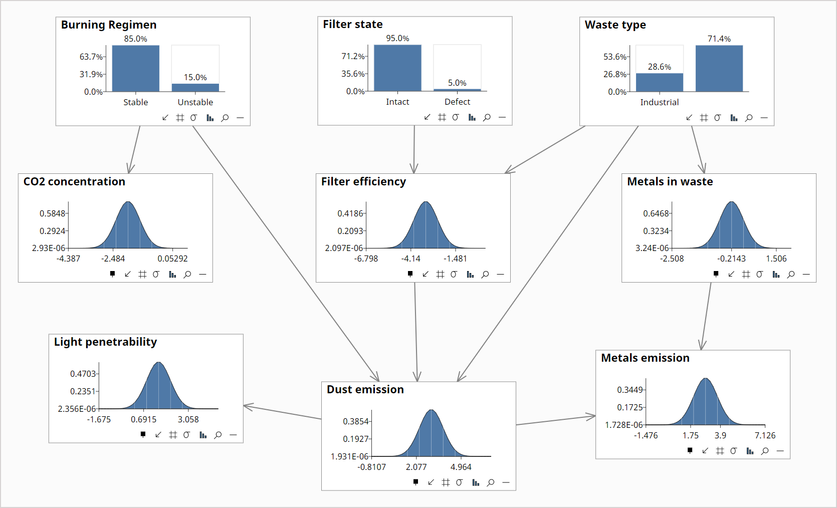
- From the Query tab on the main menu, click Add -> All Nodes.
You can also add queries by clicking an icon on the Node Toolbar. Also, when you open a network, by default all nodes are queried automatically.
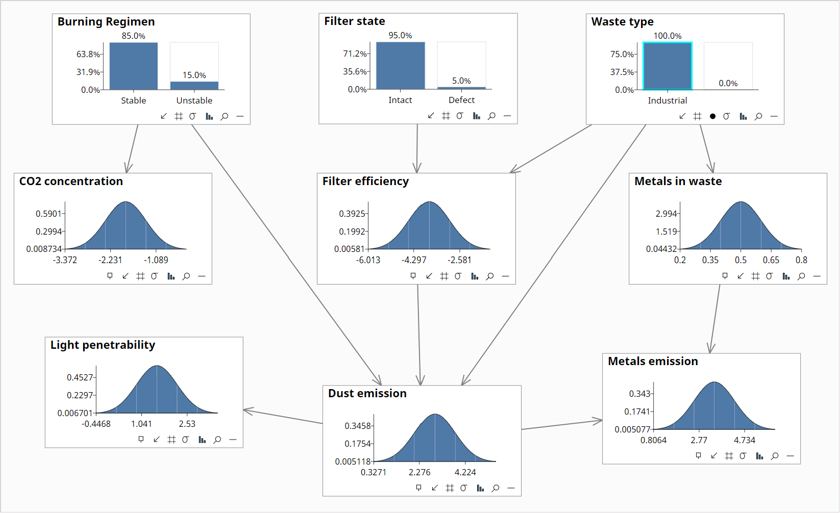
The network should look similar to the following:
- Click on the visual bar representing Waste type=Industrial to set evidence.
The network should look similar to the following: